Home / Examples / Analysis with Deformed Meshes

Analysis with Deformed Meshes

General

A capacitor is deformed due to thermal loading. The deformation causes the capacitance change.
First, the deformation due to thermal loading is calculated by the stress analysis (Galileo). Then, the capacitance is solved by the electric analysis (Coulomb) based on the deformed meshes.
The capacitances before and after the deformation are compared.
Unless specified in the list below, the default conditions will be applied.

Procedure (overview)

Select Galileo and set the analysis conditions for stress analysis.
Change the solver from Galileo to Coulomb on the [Solver] tab. Set the analysis conditions for electric field analysis.
See [Solver Tab] for the detail.
Change the solver back to stress analysis.
Execute the stress analysis and save the results.
The deformed meshes are generated and saved.
The result file containing the deformed mesh information bears (Deformed mesh) on its name.
Copy the analysis model.
Change the solver to Coulomb, which uses the deformed meshes.
On the [Model] tab 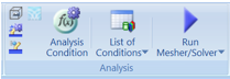, click ▼ at the bottom of [Run Mesher/Solver].

Click [Run Solver with Existing Meshes] on the submenu. Select the deformed mesh file saved in Step 2.

See [Run Solver with Existing Meshes] for more details.
The analysis procedure is as described below.
If a result file of the deformed mesh is not output, select [Save the deformed mesh results when saving the calculation result] on the GUI Setting tab in the General Settings dialog box.

Analysis Space

Items	Settings
Analysis Space	3D
Model Unit	mm

Analysis Conditions

Galileo and Coulomb are used in this session.

Items

Settings

Solver

Stress Analysis [Galileo]

Electric Analysis [Coulomb]

Analysis Type

Steady-state Analysis

The reference temperature is set on the thermal load tab.

Tab	Item	Settings
Thermal Load	Reached Temperature	200 [deg]

Model

Create a cubic solid body for the dielectric body of the capacitor. The material is alumina.

Inside the air cube, create 2 sheet bodies for electrodes. Then, specify the electric potential on each as boundary condition.

Boundary conditions for the electric analysis must be set before calculating the deformed meshes in the stress analysis.

See [Modeling] for more details.

Body Attributes and Materials

Two sheet bodies are used to imprint the electric potential-specified boundary condition.

They are called "imprinting body".

You don't need to set the body attribute or the material property on them.

Body Number/Type	Body Attribute Name	Material Name
0/Solid	Block	001_Alumina *
1/Sheet	Imprinting body
2/Sheet	Imprinting body

* Available from the Material DB

Boundary Conditions

- Stress analysis

Boundary Condition Name/Topology	Tab	Boundary Condition Type
V0/Face	Mechanical	Free *
V1/Face	Mechanical	Free *

* Free is the default setting in the stress analysis.

- Electric analysis

Boundary Condition Name/Topology	Tab	Boundary Condition Type	Settings
V0/Face	Electric	Electric Wall	Electric Potential Specified 0 [V]
V1/Face	Electric	Electric Wall	Electric Potential Specified +1 [V]

Procedure (Detailed)

Set up the analysis conditions for the stress analysis as follows.

On the [Model] tab ,

Select [Analysis Condition] .

Select the [Stress Analysis "Galileo"] on the [Solver] tab.
Click the [Stress Analysis] tab.

Select [Thermal Load]. The Thermal Load tab becomes available.
Click the Thermal Load tab.
Set 200 and 0 degrees as the reached temperature and the reference temperature, respectively and click [OK].
Set the body attribute and the material property of the body0 (solid body) as follows.
See [How to Set Body Attribute/Material Property] for detailed setup.
Set the boundary conditions on body1 and body2 (sheet bodies) as follows.
Boundary Condition Name : V0, V1 as shown in Model.
Boundary Condition : Free

See [How to Set the Boundary Condition] for the details.
Set up the analysis conditions for the electric analysis as follows.

On the [Model] tab ,

Select [Analysis Condition] .

Select [Electric Analysis "Coulomb"] on the [Solver] tab.
Click [Electric Analysis] tab.
Set it up as follows and click [OK].
Set boundary conditions on body1 and body2 (sheet bodies) as follows.
Boundary Condition Name : V0, V1 as shown in Model.
Boundary Condition : Electric Wall (Electric Potential Specified), 0V(body1), 1V(body2)
See [How to Set the Boundary Condition] for the details.
Change the solver to Stress Analysis "Galileo" as follows.

On the [Model] tab ,

Select [Analysis Condition] .

On the [Solver] tab, deselect Electric Analysis "Coulomb" and select Stress Analysis "Galileo".
Click [OK].
On the [Model] tab ,

click [Run Mesher/Solver] .
Click [Femtet] button and click [Save Project] .

Two results files (.pdt), will be saved.
The file containing deformed mesh information bears the name of "Deformed mesh".
Copy the analysis model.
Right click on "Analysis Model" on the Project tree, and click [Copy into Project].
Change the solver from Stress analysis "Galileo" to Electric analysis "Coulomb" as follows.

On the [Model] tab ,

Select [Analysis Condition] .

On the [Solver] tab, deselect Stress Analysis "Galileo" and select Electric Analysis "Coulomb".
Click [OK].
On the [Model] tab , click ▼ at the bottom of [Run Mesher/Solver].

Select [Run Solver with Existing Meshes] on the submenu.

Select the deformed mesh file saved in Step 11 for the stress analysis.

See [Run Solver with Existing Meshes] for more details.