Home / Examples / Fluid Analysis [Bernoulli] / Example 16: Capillary Action Analysis

Example 16: Capillary Action Analysis

General

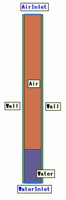
The model is two parallel plates and water sandwiched between them. Water rising by surface tension is solved with the VOF method.
The volume fractions of air and water are solved.
Unless specified in the list below, the default conditions are applied.

Results will vary depending on Femtet version and the PC environment.

Analysis Space

Item	Settings
Analysis Space	2D
Model Unit	mm

Analysis Conditions

Item

Tab

Settings

Solver

Fluid Analysis [Bernoulli]

Analysis Type

Fluid Analysis

Transient Analysis

Multiphase Flow Setting

Fluid Analysis
Multiphase Flow Setting

Execute free surface analysis (VOF method): Select

Phase Setting: Register [000_Air] and [100_Water].

Take into account weight: Select

Take into account surface tension: Select

Phase Pair Setting:

Phase 1	Phase 2	Surface Tension	Contact Angle
000_Air	100_Water	0.07	90

Detailed Settings

Fluid Analysis

Setup Details

Volume Control Type: Cell-centered Base

Timestep

Transient Analysis

Item	Settings
Timestep	Specified by 0.1 [ms]
Calculation Steps	5000
Output interval	100

Meshing Setup

Mesh

Item	Settings
General Mesh Size	Specified by 0.1 [mm]
Element Type	Rectangle

Model

Body Attributes and Materials

Body Number/Type	Body Attribute Name	Material Name
0/Face	Wall	Wall
1/Face	Wall	Wall
2/Face	Water	100_Water *
3/Face	Air	000_Air *

* Available from the material DB

The material property of “Wall” is set as follows.

Material Name	Tab	Settings
Wall	Solid/Fluid	Solid

Contact Angle is set in the body attributes of “Wall”.

Body Attribute Name

Tab

Settings

Wall

Solid

Multiphase Flow Setting (Contact Angle Setting):

Specify for each body attribute: Select

Phase Pair Setting:

Phase 1	Phase 2	Contact Angle
000_Air	100_Water	60

Boundary Condition

Boundary Condition Name/Topology

Tab

Boundary Condition Type

Settings

WaterInlet/Edge

Fluid

Inlet/Outlet

Natural Inflow/ Natural Outflow

Multiphase Flow Setting:

Inflow Phase [100_Water]

AirInlet/Edge

Fluid

Inlet/Outlet

Natural Inflow/ Natural Outflow

Multiphase Flow Setting:

Inflow Phase [000_Air]

Results

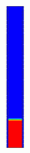
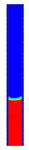
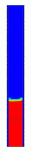
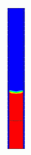
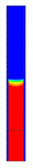
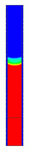
The volume fraction contours of phase 2 at 0, 0.1 [s], 0.2 [s], 0.3 [s], 0.4 [s], and 0.5 [s] are shown below.

Phase 2 (Water) is indicated in red.

Water level rises until 0.4 [s] and then decreases at 0.5 [s].

The water level does not converge to a certain value.

Time: 0 [s]	Time: 0.1 [s]	Time: 0.2 [s]	Time: 0.3 [s]	Time: 0.4 [s]	Time: 0.5 [s]

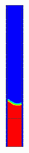
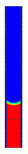
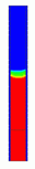
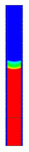
With contact angles taken into account, the calculation may not converge due to boundary oscillations.

About 10 times larger viscosity can suppress the undesired oscillations.

The steady-state is calculated where the surface tension and the weight are balanced.
Then, the change in viscosity does not affect the calculation of the steady-state.

Water level can be obtained from the equations below, which indicates water level does not depend on viscosity.

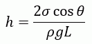
H [m]: Water Level, σ [N/m]: Surface Tension Coefficient, θ: Contact Angle, ρ [kg/m3]: Water Density, g [m/s2]: Gravitational Acceleration, L [m]: Distance between the parallel plates

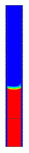
The calculation results with 10 times higher viscosity are shown below.

Water level converges to a certain value.

Time: 0 [s]	Time: 0.1 [s]	Time: 0.2 [s]	Time: 0.3 [s]	Time: 0.4 [s]	Time: 0.5 [s]

The water levels of the two models are acquired by [VOF CaptureBoundary Macro.xlsm] and shown in the graph below.

The water level converges to about 5.8 [mm].

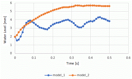
The theoretical value of water level is,

h = 2 * 0.07 * 0.5 / (997 * 9.8 * 0.1e-3 ) = 7.16 [mm].

The theoretical water level is slightly higher than the calculated level.