General
Home / Examples / Electromagnetic Analysis [Hertz] / Example 24: Waveguide-to-Coaxial Adapter
The characteristics of a waveguide-to-coaxial adapter are analyzed.
How to analyze a cylindrical waveguide is explained.
Unless specified in the list below, the default conditions will be applied.
Results will vary depending on Femtet version and the PC environment.
The harmonic analysis is set as follows.
Tab |
Setting Item |
Settings |
Mesh Tab |
Frequency-Dependent Meshing |
Reference Frequency: 1x10¹⁰ [Hz] Select [The conductor bodies thicker than the skin depth constitute the boundary condition].
|
Harmonic Analysis |
Sweep Type |
Select [Linear Step by Division Number] |
Sweep Setting |
Minimum: 8×10⁹ [Hz] Maximum: 15x109 [Hz] Division: 7 |
|
Sweep Setting |
Select Discrete Sweep |
|
Input |
1.0 [W] |
The model is a waveguide-to-coaxial adapter. The inner conductor of coaxial cable is penetrated into the circular waveguide.

Body Number/Type |
Body Attribute Name |
Material Name |
7/Solid |
InnerConductor |
003_Ag * |
8/Solid |
Waveguide |
000_Air(*) |
9/Solid |
Resin |
Resin |
* Available from the material DB
The material properties of Resin are set up as follows:
Material Name |
Tab |
Properties |
DRMat |
Permittivity |
Relative Permittivity: 2.3
|
Boundary Condition Name/Topology |
Tab |
Boundary Condition Type |
Settings |
Port_001/Face
|
Electric |
Port
|
Reference Impedance: Specify enter 50 ohms Number of Modes Number of Precalculated Modes: 5 Number of Modes Used in the Actual 3D Analysis: 1 Select modes: None |
Port_002/Face |
Electric |
Port |
Reference Impedance:
Number of Modes Number of Precalculated Modes: 5 Number of Modes Used in the Actual 3D Analysis: 2 Select Modes: None |
Outer Boundary Condition |
Electric |
Electric Wall |
|
Notes:
The number of modes used in the actual analysis is 2 for Port_002.
This is because the electromagnetic solver has two modes corresponding to the TE11 modes which are the basic mode of the cylindrical waveguide.
As shown in Figure 1, the directions of their electric field vectors are angled 90 degrees each other.
The two modes must be used in order to perform analysis taking TE mode into account. Currently, Femtet cannot control the direction of electric field of mode.
The port numbers are automatically assigned by the port name and the number of modes used for analysis.
Ports have been set as follows.
Port_001 “Number of modes used in the actual analysis”: 1
Port_002 “Number of modes used in the actual analysis”: 2
Therefore, S-parameters are a 3 x 3 matrix.
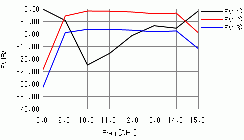
Fig. 1 Frequency Response of S-parameters
On the Results tab, click [Chart] - [SYZ Matrix]. The following will appear.
| Port Index |
| 1:Port_001:m1 |
| 2:Port_002:m1 |
| 3:Port_002:m2 |
"m1" and "m2" indicate the mode number.
See [How to Examine the Ports of Electromagnetic Analysis] for the detail.
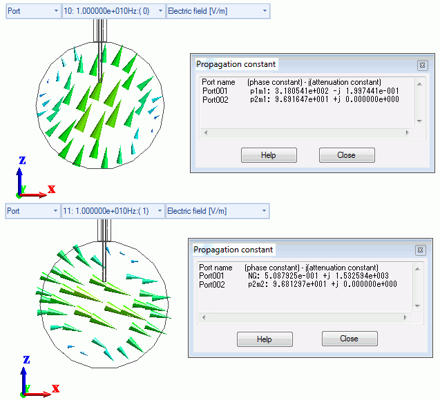
Fig. 2 Distribution of Electric Field of Two Propagation Modes Corresponding to TE11 Modes
The first propagation constant dialog box above shows the following:
(This dialog box appears when you click [Chart] - [Mode Information] on the Results tab  )
)
Port_002 p2m1: 9.691647e+001 +j 0.000000e+000
This is for Port_002:m1 of Port Index.
Note that "p" is for port and "m" is for mode in p2m1. The second "propagation constant" dialog box shows the following:
PORT2_002 p2m2: 9.681297e+001 +j 0.000000e+000
This is for Port_002:m2 of Port Index.
The power entered at Port_001 reaches Port_002 in these two modes.
The total power is acquired by the following equation.
Please use Excel or any other tool to calculate it. Femtet doesn't calculate this equation.
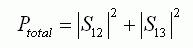 (1)
(1)
Please also keep in mind the following point.
A TM01 mode also propagates at 12 [GHz] or higher. For better accuracy at 12 [GHz] or higher,
increase [Number of modes used in the actual 3D analysis] for Port_002 from 2 to 3.
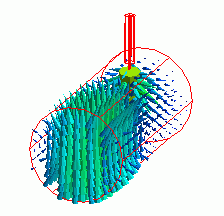
Fig. 3 shows that TM01 can propagate.
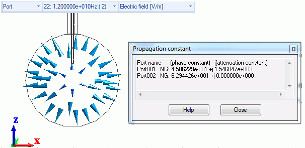
Fig. 3 TM0-Mode Electric Field Distribution (at 12 GHz)