Home / Examples / Acoustic Analysis [Mach] / Example 1: Radiation Impedance of Disc
A vibrating disc is placed in the air. The sound waves generated by it are analyzed.
The sound power, the radiation impedance and the sound pressure distribution for each frequency are solved.
Unless specified in the list below, the default conditions will be applied.
Results will vary depending on Femtet version and the PC environment.
Item |
Settings |
Analysis Space |
3D |
Model unit |
m |
Item |
Settings |
Solver |
Acoustic Analysis [Mach] |
Analysis Type |
Harmonic analysis |
Options |
N/A |
The harmonic analysis tab is set up as follows.
The sound waves propagate outside the analysis region. Therefore the "open boundary" condition below is applied initially.
The default conditions will be applied.
Tabs |
Setting Item |
Settings |
Harmonic analysis
|
Frequency |
Minimum: 200[Hz] Maximum: 3000[Hz] |
Sweep Type |
Select Linear Step by Division Number. Division: 20 |
|
Sweep Setting |
Select Fast sweep. Tolerance: 1.0x10⁻² |
|
Open Boundary Tab |
Type |
Absorbing boundary |
Order of Absorbing Boundary |
1st order |
|
Coordinates of Origin |
x = y = z = 0 |
The air hemisphere is created from a solid body.
The open boundary is set on the surface of the hemisphere. A circular sheet body is defined for imprinting.
The velocity boundary condition is applied.
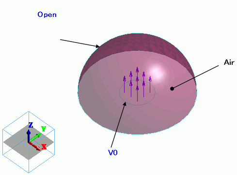
The hemispheric solid body is created. The material is air.
The "speed" boundary condition is set on the circular face topology, which is created by segmenting the circular sheet body.
Body Number/Type |
Body Attribute Name |
Material Name |
0/Solid |
Air |
000_Air(*) |
* Available from the material DB
The [speed] boundary condition is set on the face of the imprinting body.
Boundary Condition Name/Topology |
Tab |
Boundary Condition Type |
Settings |
Open/Face |
Acoustic |
Open boundary |
|
V0/Face |
Acoustic |
Speed |
1[m/s] |
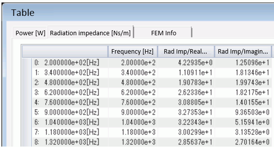
To see the calculated characteristics, go to the [Results] tab,

and click [Table]![]() .
.
As an example, radiation impedance is shown below. The graph can be displayed as well, by pressing the [Graph] button at the bottom of the table.
Other characteristics can be seen on other tabs.
The results and the theoretical values match. The theoretical values are calculated and plotted by Excel.
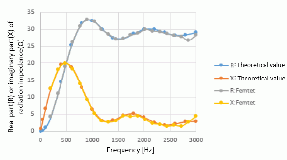
The theoretical values are calculated by the equations below. (*)
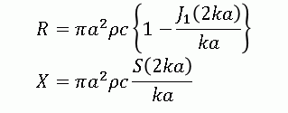
R: real part of the radiation impedance, X: imaginary part of the radiation impedance,
a: radius of the driving source, ρ: air density, c: sound speed, k: wavenumber (=2π/wavelength),
J1(z): 1st-order Bessel function
S(z): Struve function
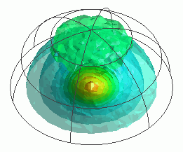
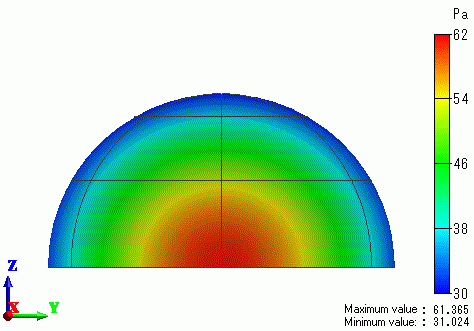
The gradation contour of the sound pressure at the driving frequency of 200[Hz]
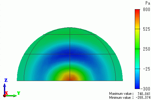
The gradation contour of the sound pressure at the driving frequency of 900[Hz]
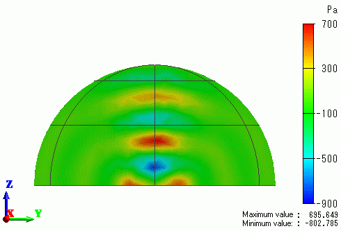
The gradation contour of the sound pressure at the driving frequency of 2020[Hz]
The gradation contour of the sound pressure at the driving frequency of 3000[Hz]
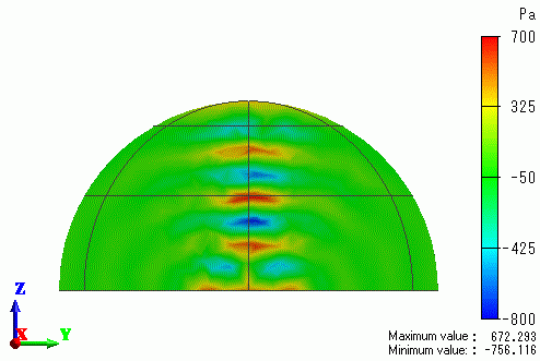
The sound pressure varies as the driving frequency changes.