General
Home / Examples / Acoustic Analysis [Mach] / Example 2: Directivity of Disc
A vibrating disc is placed on an infinite plate. The sound waves generated by the disc are analyzed.
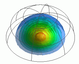
The sound pressure levels are calculated on the surface of a hemisphere, at the specified distance from the disc. The radiation patterns are solved.
Unless specified in the list below, the default conditions will be applied.
Results will vary depending on Femtet version and the PC environment.
Item |
Settings |
Analysis Space |
3D |
Model Unit |
m |
Item |
Settings |
Solver |
Acoustic Analysis [Mach] |
Analysis Type |
Harmonic Analysis |
Options |
N/A |
The harmonic analysis tab is set up as follows.
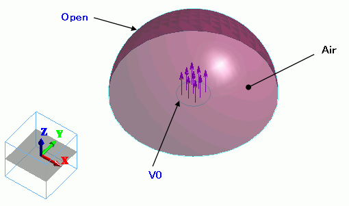
The sound waves propagate outside the analysis region. Therefore the [Open Boundary] condition below is applied initially.
The default conditions will be applied.
Tabs |
Setting Item |
Settings |
Harmonic analysis
|
Frequency |
Minimum: 52.7 [Hz] Maximum: 52.7*5 [Hz] |
Sweep Type |
Select Linear Step by Division Number. Division: 2 |
|
Sweep Setting |
Select Fast Sweep. Tolerance: 1.0x10⁻² |
|
Open Boundary Tab |
Type |
Absorbing Boundary |
Order of Absorbing Boundary |
1st-order |
|
Coordinates of Origin |
x = y = z = 0 |
The air hemisphere is created from a solid body. The [Open Boundary] is set on the surface of the hemisphere.
The [speed] boundary condition is set on the circular face topology, which is created by creating a circular sheet body and segmenting it.
Body Number/Type |
Body Attribute Name |
Material Name |
0/Solid |
Air |
000_Air(*) |
* Available from the Material DB
The [Speed] boundary condition is set on the face of the imprinting body.
Boundary Condition Name/Topology |
Tab |
Boundary Condition Type |
Settings |
Open/Face |
Acoustic |
Open Boundary |
|
V0/Face |
Acoustic |
Speed |
1 [m/s] |
The sound pressures at the points distanced 100 m away from the origin are solved and the directivities are shown below.
On the [Results] tab  , click ▼ at the side of
 ![]() , and select Directivity.
, and select Directivity.
The [Directivity Calculation] dialog box will show up.
Set it up as follows, and press the Polar Graph button. The directivity will be shown in polar graph for each frequency.
Select XY plane of symmetry to calculate the infinite plane.
Item |
Settings |
Mode: Frequency [Hz] |
Select the mode to display. |
Observation Point |
r: 100 [m] φ: Enter 0 in all
θ: Max 90 [deg] Step 60 |
Display |
Sound Pressure Level [dB] |
Plane of Symmetry |
XY plane |
The polar graph of directivity at the driving frequency of 263.5 [Hz] is as follows.

The graphs at the frequencies are displayed overlaid. The theoretical graph is also displayed overlaid. The calculation results and the theoretical values match very well.
See here for how to add data to the graph.

The theoretical value of the radiated sound pressure [Pa] is derived from the following equation. The unit is converted from Pa to dB as shown above.
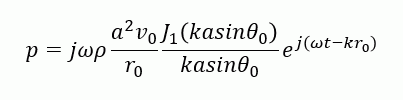
where p: sound pressure, ω: angular frequency, ρ: density, a: radius of driving disc, k: wavenumber, θ0: observation direction (angle from Z axis)
V0: amplitude of velocity of driving source, r0: distance to the observation point, t: time, j: unit of imaginary number