
Home / Examples / Piezoelectric Analysis [Rayleigh] / Example 11: Transient Analysis
Transient analysis is explained in this example.
As a result, the displacement change over the time can be viewed.
Unless specified in the list below, the default conditions will be applied.
Results will vary depending on Femtet version and the PC environment.
Transient analysis is available in an optional package. However, transient analysis using resonant mode is not optional.
Item |
Settings |
Analysis Space |
3D |
Model Unit |
mm |
Item |
Settings |
Solver |
Piezoelectric Analysis [Rayleigh] |
Analysis Type |
Transient Analysis |
Transient Analysis Using Resonant Mode (Model 1) |
Deselected |
Transient Analysis Using Resonant Mode (Model 2)
|
Selected
|
The settings on the transient analysis tab are required.
For model 2, settings on the resonant analysis tab are required.
The resonant and transient analysis tabs are set up as follows.
Tab |
Setting Item |
Settings |
Mesh |
Order of Element | 1st-order Element (Time Prioritized) |
Resonant Analysis (only for model 2) |
Number of Modes |
10 |
Approximated Frequency |
0 [Hz] |
|
Transient Analysis |
Timestep |
Select [Specify] |
Output Interval |
5 |
|
Calculation Steps |
1000 |

Body Number/Type |
Body Attribute Name |
Material Name |
0/Solid |
piezo |
000_P-4 * |
* Available from the material DB
The time dependency of the applied voltage is defined by weight function.
Boundary Condition Name/Topology |
Tab |
Boundary Condition Type |
Settings |
earth/Face |
Electric |
Electric Wall |
Specify electric potential: Electric Potential 0 [V] |
Mechanical |
Displacement |
Select UZ only UZ=0 |
|
hot/Face |
Electric |
Electric Wall |
Specify electric potential: Electric Potential 1 [V] Select [Time Dependency]. Define weight function. |
Mechanical |
Free |
|
|
UX0/Face
|
Electric |
Magnetic Wall |
|
Mechanical |
Displacement |
Select UX only UX=0 |
|
UY0/Face |
Electric |
Magnetic Wall |
|
Mechanical |
Displacement |
Select UY UY=0 |
The weight function set for the boundary condition of “hot” is plotted below.

The vibration is compared between models 1 and 2.
The diagram below is time response at the coordinates (2.5, 0.0, 0.1). The results of models 1 and 2 are plotted on the same graph.
See [Field Graph] for more details.
To see the time response, click [Results] > [Select Solver] and select [Piezo/Time response].
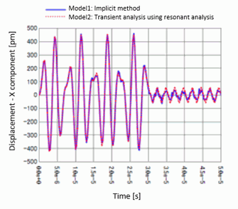
The voltage is constant at 0 [V] after 30 [us] and the change in displacement response is observed.