Home / Examples / Electromagnetic Analysis [Hertz] / Example 45: Radar Cross Section (RCS) of Conductive Sphere

Example 45: Radar Cross Section (RCS) of Conductive Sphere

 

General

• Femtet can not calculate Radar Cross Section (RCS) directly. However, with additional calculations, RCS can be easily solved.
  

• The example is a canonical problem provided by the Electronics Society of IEICE in Japan.
   

• Unless specified in the list below, the default conditions are applied.
  

• Obtain this session's project file. (Right-click and choose 'Save link as')




• Results will vary depending on Femtet version and the PC environment.

Analysis Conditions

Item	Settings
Solver	Electromagnetic Analysis [Hertz]
Analysis Space	3D
Analysis Type	Harmonic Analysis
Unit	mm
Analysis Options	Select [Ignore the influence of face/edge electrode thickness] *

* This option is selected be by default. In this example, the results will not be affected if it is deselected because there is no face electrode.

 

The Harmonic Analysis tab and Open Boundary tab are set as follows.

Tab	Setting Item	Settings
Harmonic Analysis	Frequency	Single Frequency 2.998 [GHz]
	Sweep Setting	Discrete Sweep
	Input	1.0 [W]
Incident Wave (plane wave)	Propagation Direction	( 0, 0, 1)
	Electric Field Vector	( 1, 0, 0) [V/m]
Open Boundary	Type	Absorbing Boundary
	Order of Absorbing Boundary	1st-order

 

Model

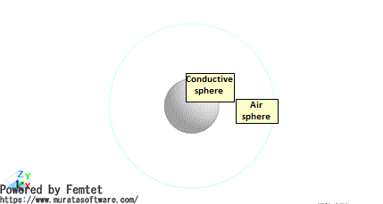
The model inludes a body of air and a body of a conductive sphere. The Open Boundary condition is set using the Outer Boundary condition.

 

 

 

 

Body Attributes and Materials

Body Number/Type	Body Attribute Name	Material Name
0/Solid	Conductive Sphere	008_Cu *
1/Solid	AIR Sphere	000_Air *

* Available from the material DB

 

Boundary Conditions

Boundary Condition Name/Topology	Tab	Boundary Condition Type	Settings
Outer Boundary Condition	Electric	Open Boundary

 

Set up Mesher/Solver

Setting Item	Settings
Frequency-Dependent Meshing	Reference frequency: 2.998 [GHz] Select The conductor bodies thicker than the skin depth constitute the boundary condition

Since Metal is thicker than the skin depth in the setting, the surface of Metal is set with the boundary condition of copper material loss.

 

Results

Femtet can not calculate Radar Cross Section (RCS) directly. However, with additional calculations, RCS can be easily solved.

The equation of RCS(σ) is as follows.

 R: Observation Point (Distance from Origin)

 ES: Electric Field of Scattered Wave

 Ei: Electric Field of Incident Wave

 

 

RCS[dBsw]（=σdBsw）, which is normalized by the wavelength (λ) in vacuum, can be obtained from the equation below. To calculate the equation with R approaching infinity, the condition that the observation point is sufficiently far away from the origin is taken into account.

 ES and Ei are effective values. The equation is as follows.

 

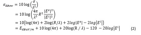
"Log" is the common logarithm.

On the right side of Equation (2), the first term is solved with the surrounding electromagnetic field calculation in Femtet.

As each term from the second term on the right side of Equation (2) is easily calculated, adding them can result in RCS [dBsw]. In Femtet, direct calculation is not possible; instead, Excel is used.

The fourth term (-120) on the right side of Equation (2) appears when the unit is dBuV/m. See the bottom of this page for more details about the unit.

 

• Amplitude is entered on the Incident Wave (Plane Wave) tab in the Analysis Condition Setting dialog box. Be aware that the fifth term, Ei, on the right side of Equation (2) is the effective values.

 

Substituting the values below for Equation (2) will give Equation (3).

  Ei = 1/1.414 [V/m]: Effective value of the electric field of the incident wave.

 λ=0.1 [m]:   Wavelength at 2.998 [GHz] in vacuum

  R=3.0 [m]: Observation point. This corresponds to the observation point, r, in the surrounding electromagnetic field dialog box. The value of 3.0 [m] is 30 times as long as the wavelength. It is a sufficiently far distance.

 

 

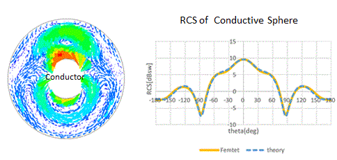
The electromagnetic field distribution obtained in the electromagnetic analysis is shown below.

 

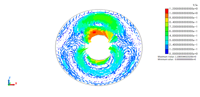
Fig.1 Electromagnetic Field Distribution

 

Firstly, E [dBuV/m] is solved using the surrounding electromagnetic field calculation

The component of Eθ is calculated here.

 

 

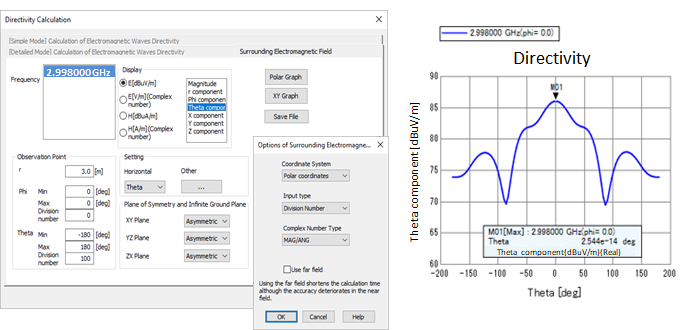
Fig. 2 Directivity Calculation dialog, Surrounding Electromagnetic Field tab Fig. 3 Eθ [dBμV/m] from the surrounding electromagnetic field calculation

 

 

 

 

 

The graph below shows the result obtained by saving the surrounding electromagnetic field into a csv file and then performing the calculation of Equation (3) with Excel. The results of the numerical analysis and theoretical calculation match well.

 

 

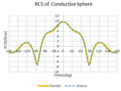
Fig. 4 RCS [dBsw] of Conductive Sphere ,created with Excel.

 

 

 

 

[Appendix]

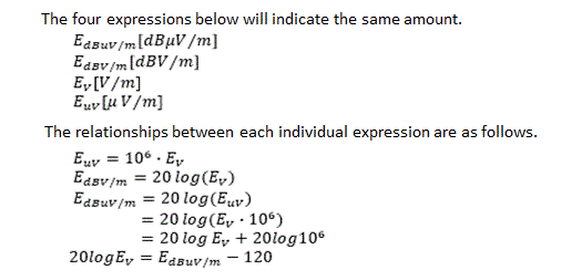
Refer below for unit conversion.