


|
Home / Examples / Acoustic Analysis [Mach] / Example 16: Speed Boundary Condition
Example 16: Speed Boundary Condition
General
-
The speed boundary condition is set up here.
-
If the speed boundary condition is set inside the analysis model, select [Discontinuous] additionally.
-
Unless specified in the list below, the default conditions will be applied.
-
Obtain this session's project file. (Right-click and choose 'Save link as')
Analysis Space
|
Item |
Settings |
|
Analysis Space |
2D |
|
Model Unit |
mm |
|
Thickness in Depth Direction |
1.0 [mm] |
Analysis Conditions
|
Item |
Settings |
|
Solver |
Acoustic Analysis [Mach] |
|
Analysis Type |
Harmonic Analysis |
|
Tab |
Setting Item |
Settings |
|
Harmonic Analysis |
Frequency |
1 freq only 1000 [Hz] |
Model
Three models are applied.
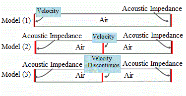
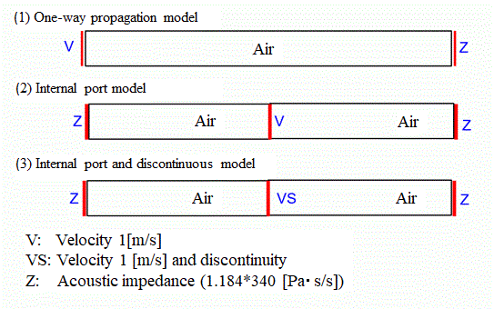
(1) Sound travels through the pipe. Set the speed boundary condition at the left end of the pipe. It drives sound vibrations.
Sound propagates through the pipe and exits at the right end. To prevent sound from reflecting, the specific acoustic impedance of the medium is set at the right end of the pipe.
The size of the pipe is 300 by 30 [mm].
(2) Speed boundary condition is set at the middle of the pipe. To prevent sound from reflecting, the acoustic impedance of the medium is set at both ends of the pipe. The size of the pipe is 600 by 30 [mm].
(3) [Discontinuous] is additionally selected for the speed boundary of (2). The size of the pipe is 600 by 30 [mm].
Body Attribute and Material Property Setting
|
Body Number/Type |
Body Attribute Name |
Material Name |
|
0/Sheet |
Body_Attribute_001 |
000_Air * |
* Available from the material DB
Boundary Conditions
|
Boundary Condition Name/Topology |
Tab |
Boundary Condition Type |
Settings |
|
V/Edge |
Acoustic |
Speed |
1 [m/s] |
|
Symmetry/Continuity |
---- |
|
|
|
Z/Edge |
Acoustic |
Acoustic Impedance |
1.184* 340 [Pa*s/m] |
|
Symmetry/Continuity |
---- |
|
|
|
VS/Edge |
Acoustic |
Speed |
1 [m/s] |
|
Symmetry/Continuity |
Discontinuous |
||
|
Outer Boundary Condition * |
Acoustic |
Rigid Body |
|
|
Symmetry/Continuity |
---- |
|
* Set the specific acoustic impedance of air. It can prevent sound reflection.
Results
First, examine the results of the simple one-way propagation model (model (1)).
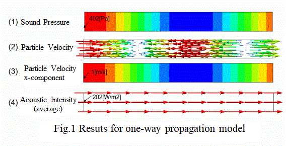
Since the speed is set to 1 [m/s], the x-component of the particle velocity of the result fields is observed as 1 [m/s].
For a sound wave traveling unidirectionally, the relationship (sound pressure = particle velocity x specific acoustic impedance) must be satisfied.
As the specific acoustic impedance of air is given as 1.184*340=402.56 [Pa・s/m], the sound pressure is expected to be 402 [Pa].
The estimated sound pressure can be verified in Fig. 1 (1).
Fig. 2 shows the temporal changes in sound pressure and the x-component of particle velocity at the left end of the model (the position of the sound boundary), displayed as a graph over one period.
The horizontal axis represents the phase. Viewing the graph over 360 degrees of phase corresponds to observing one full period.
Both sound pressure and particle velocity reach their maximum at a phase of 0 degrees and their minimum at 180 degrees, indicating that they vibrate in phase.
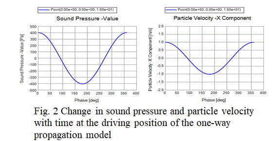
Fig. 3 shows the result of the internal port model (model (2)).
The x-component of particle velocity is shown both as a contour diagram and as a graph, where the horizontal axis of the graph represents the position along the longitudinal direction of the contour diagram.
The particle velocity changes discontinuously at the speed boundary position. For the contour shown here, averaging is turned OFF in the contour settings for visualization.
The graph shows a discontinuity at the center and an amplitude of 0.5 [m/s]. This is different from 1 [m/s], which is specified as the boundary condition.
When a speed boundary condition is set inside the analysis domain, the resultant speed will not follow the specified value. The following model (model (3)) will solve the problem.
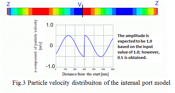
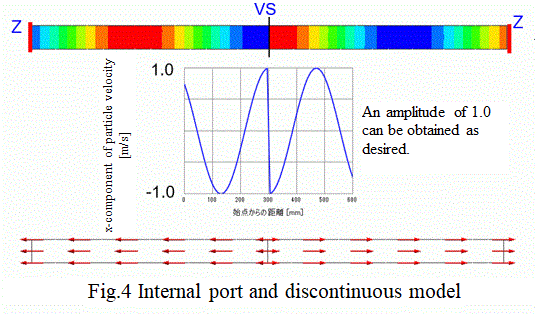
Fig. 4 shows the results of the combined model of the internal port and discontinuous models (model (3)). Both the speed and discontinuous boundary conditions are set.
The contour diagram and graph in Fig. 4 are set in the same way as in Fig. 3, indicating the x-component of particle velocity.
The vectors represent the acoustic Intensity (average). It is observed that the energy flows equally in both the leftward and rightward directions from the speed boundary.
The graph shows a discontinuity at the center and an amplitude of 1.0 [m/s]. By using both speed and discontinuous boundary conditions, the values specified by users can be properly reflected in the results.
Summary
It is verified that when a speed boundary condition is set inside the analysis domain, the resultant speed does not follow the specified value.
However, It is also verified that by combining it with a discontinuous boundary condition, the resultant speed can follow the specified value.