


|
Home / Examples / Acoustic Analysis [Mach] / Example 18: Scattering from Rigid Sphere
Example 18: Scattering from Rigid Sphere
General
-
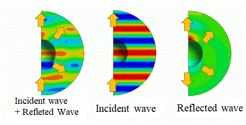
Apply plane waves.
-
The reflected wave from the rigid sphere is compared with the theoretical wave.
-
Obtain this session's project file. (Right-click and choose 'Save link as')
Analysis Space
|
Item |
Settings |
|
Analysis Space |
3D |
|
Model Unit |
m |
Analysis Conditions
|
Item |
Settings |
|
Solver |
Acoustic Analysis |
|
Analysis Type |
Harmonic Analysis |
|
Options |
Incident Wave |
|
Tab |
Item |
Settings |
|
Harmonic Analysis |
Frequency |
Single Frequency 200 [Hz] |
|
Frequency Sweep |
Single Frequency |
|
|
Options |
Select [Enable each port's individual weight setting for the field display]. |
|
|
|
|
|
|
Incident Wave (plane wave) |
Propagation Direction |
(0, 0, 1) |
|
Pressure (Sound Pressure) |
1 [Pa] Select [Sound Pressure [Pa]]. |
Model
A hole is provided in the body of air. The hole does not need any setting. It is treated as a rigid wall, which has been set for the outer boundary condition.
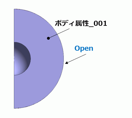
Body Attribute and Material Property Setting
|
Body Number/Type |
Body Attribute Name |
Material Name |
|
Body 4/Solid body |
Body_Attribute_001 |
000_Air * |
* Available from the material DB
Boundary Conditions
|
Boundary Condition Name/Topology |
Tab |
Boundary Condition Type |
Settings |
|
Open/Face |
Acoustic |
Open Boundary |
|
|
Outer Boundary Condition |
Acoustic |
Rigid Wall |
|
Results
How to separate incident and reflected waves, shown at the top of this page, is explained below.
Operations follow as shown in Example 17. Fig. 1 shows the sound pressure distribution [Pa] at a phase of 0 deg.
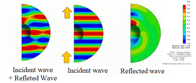
Fig. 1 Result Field Displays (sound pressure at phase of 0 deg)
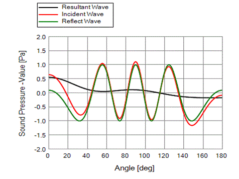
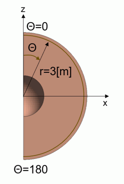
Fig. 2 Result Field Graph (sound pressure at phase of 0 deg)
Using the contour diagram in Fig. 1, Fig. 2 is plotted with Θ as the horizontal axis.
The coordinate system is displayed on the right side of Fig. 2. The graph with Θ as its horizontal axis is created under the condition that the distance from the center of the sphere is 3 m.
(To draw the graph, select [On Arc] for the location for evaluation in the Graph Setting dialog box.) The Graph Setting dialog box is explainedhere.
Next, we compare the results with the theoretical values. The synthetic wave, resulting from the incident and reflected waves, is expressed by the theoretical formula below. [1]

r,Θ: Observation Point
k: Wavenumber
a: Radius of rigid sphere
P0: Amplitude of incident wave
jn(x): Spherical Bessel function
hn(x): Hankel function of the first kind
Pn(x): Legendre polynominal
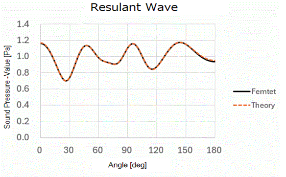
Fig. 3 Comparison of absolute sound pressure results with theoretical values
Fig. 3 is created using Excel.