|
Home / Examples / Coupled Analysis / Piezoelectric-Acoustic Analysis [Rayleigh/Mach] / Example 6: Mass Law
Example 6: Mass Law (Piezoelectric-Acoustic Coupled Analysis)
General
-
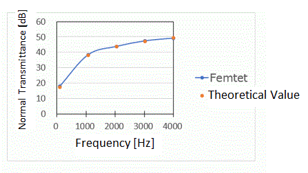
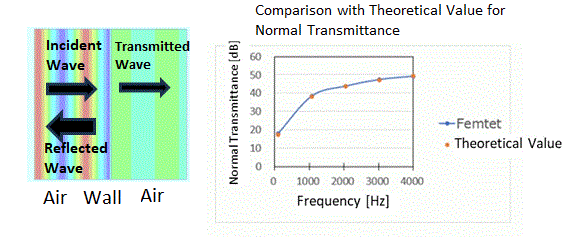
The frequency response of the wall’s transmittance is solved.
-
Obtain this session's project file. (Right-click and choose 'Save link as')
-
Results will vary depending on Femtet version and the PC environment.
Analysis Space
|
Item |
Settings |
|
Analysis Space |
2D |
|
Model Unit |
m |
|
Thickness in Depth direction |
1.0 [m] |
Analysis Conditions
The solvers are Rayleigh and Mach.
|
Item |
Settings |
|
Solver |
Piezoelectric Analysis [Rayleigh] Acoustic Analysis [Mach] |
|
Analysis Type |
Harmonic Analysis |
|
Analysis Plane |
2D Section |
|
Variables to Constrain |
Select [Electric Potential] and [Y Displacement] * |
|
Analysis Options |
Select [Fully-coupled Analysis] |
|
Output Setting |
Select [Calculate loss (Acoustic Analysis domain)] |
* To exclude piezoelectricity from the analysis, constrain the electric potential.
|
Tab |
Setting Item |
Settings |
|
Harmonic Analysis |
Frequency |
Minimum: 100 [Hz] Maximum: 4000 [Hz] |
|
Interval |
Number of Divisions: 4 |
Model
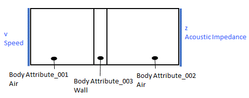
A wall is placed between air bodies.
Body Attribute and Material Setting
|
Body Number/Type |
Body Attribute Name |
Material Name |
|
0/Solid |
AIR |
000_Air * |
|
1/Solid |
WALL |
Wall |
|
2/Solid |
AIR |
000_Air * |
* Available from the material DB
|
Material Name |
Tab |
Material Name |
|
Wall |
Density |
1000 [kg/m3] |
|
Piezoelectricity |
Material Type: Perfect Conductor Anisotropy: Isotropic Young's Modulus: 206[GPa] Poisson's Ratio: 0.28 |
|
Body Attribute Name |
Analysis Domain (Solver) |
|
AIR |
Acoustic Analysis (Mach) |
|
WALL |
Piezoelectric Analysis (Rayleigh) |
Cautions: Note for the piezoelectric acoustic coupled analysis
The body to be analyzed must be specified to be subject to the piezoelectric or acoustic analysis. That is, in the analysis domain tab, either Piezoelectric Analysis or Acoustic Analysis must be selected.
Boundary Conditions
|
Boundary Condition Name/Topology |
Tab |
Boundary Condition Type |
Settings |
|
v/Edge |
Acoustic |
Speed
|
1 [m/s] Select [Specify the incident wave] |
|
z/Edge |
Acoustic |
Acoustic Impedance |
402.56[Pa・s/m] * |
* Set the specific acoustic impedance of air.
Results
The resultant distribution of sound pressure at 1.075e+03 [Hz] is shown below. Confirm the analysis type of the result filed is the acoustic analysis.
The contour diagram is illustrated using the setting below.
| Acoustic Analysis | 1: 1.075000E+3 [Hz] |
| Sound pressure [Pa] | Value |
| 0 [deg] | Linear |
Table 1. Setting in Result Field for Fig. 1
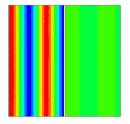
Fig. 1 Sound Pressure Distribution 1.075 [kHz]
Calculate the transmittance (T). The equation below will give the transmittance.
T = It/Ii
It: Can be acquired on the [Loss at Boundary] tab in the result table.
Ii: Can be acquired on the [Input Power] tab in the result table.
Calculate using the results from Femtet.
The results at 100 [Hz] are shown below.
Ii = 3.25 [W]
It = 201.28 [W]
-10・Log(3.25/201.2) = 17.9 [dB]
Calculation of theoretical values
20・Log(f・m) - 42.5 = 17.5 [dB]
Mass: m = 10 [kg], calculated from the width of the wall, 1 [cm], the thickness in the depth direction, 1 [m], and the density, 1000 [kg/m3] of the analysis model.
Frequency: f = 100 [Hz]