Home / Examples / Coupled Analysis / Piezoelectric-Acoustic Analysis [Rayleigh/Mach] / Example 4: Transient Analysis

Example 4: Transient Analysis

General

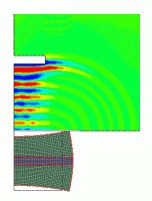
This is a transient analysis of piezoelectric-acoustic coupled analysis. The piezoelectric solver executes transient analysis using resonant mode.
A piezoelectric material is driven by voltage to generate sound wave propagation.
Obtain this session's project file. (Right-click and choose 'Save link as')
(The analysis model with the timestep adjusted automatically is also included in the project file)
Results will vary depending on Femtet version and the PC environment.

Unless specified in the list below, the default conditions will be applied.

Analysis Conditions

Item	Settings
Solver	Piezoelectric Analysis [Rayleigh] Acoustic Analysis [Mach]
Analysis Space	2D
Analysis Type	Transient Analysis
Unit	mm
Transient Analysis Using Resonant Mode	Selected

In the piezoelectric-acoustic coupled analysis, it is not allowed to deselect transient analysis that uses resonant mode.

Tab

Setting Item

Settings

Mesh

Meshing Setup

Element Type: Rectangle

☑ Square or close in shape

Resonant Analysis

Number of Modes: 3

Approximated Frequency: 0

Transient Analysis (Timestep: Manual)

Timestep

Manual

No	Number of Calculation Steps	Output Interval	Timestep [s]
1	250	1	2.0e-6

Solution Method (Acoustic Analysis)

Implicit Method

Transient Analysis (Timestep: Automatic)

Timestep

Automatic

Finish Time

0.5 [s]

Number of calculation steps

1000

Solution Method (Acoustic Analysis)

Implicit Method

The timestep is determined based on the resonant frequency and the applied frequency. The resonance at 41 kHz is confirmed by a resonant analysis performed in advance. Based on it, the applied frequency is set at 40 kHz, which is slightly lower than the resonance.
At 40 kHz, the period T0 is T0=1/40e3=2.5e-5. Timestep (dT) is required to be or less than 1/10 of the period. So the value is set to dT=2.0e-6[s], which is slightly smaller than 1/10 of the period.
Finish time of calculation is 250 x 2.0e-6=5e-4 [s]=500 [us]. A driving frequency is required when setting the electric potential-specified boundary condition.
If auto timestep setting, the timestep will be one-tenth of the period corresponding to the maximum resonant frequency given by the resonant analysis. The number of divisions can be changed.

Model

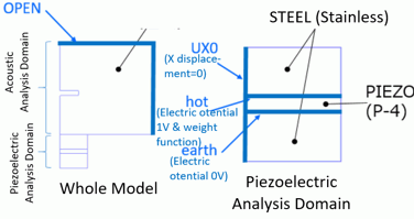
The model is a half model in 2D.

The domain for the piezoelectric analysis consists of an piezoelectric material and stainless steel. The electric potential-specified boundary conditions of hot and earth are set to the piezoelectric material. The electric potential 0 [V] is set to "earth" and the voltage oscillating in sine wave is set to "hot".

On the edge of X=0, a boundary condition with X displacement of zero is set.

The domain for acoustic analysis is air. The open boundary condition is set to the domain for the acoustic analysis.

Body Attributes and Materials

Body Number/Type	Body Attribute Name	Material Name
0/Sheet	STEEL	104_Stainless_steel *
1/Sheet	PIEZO	000_P4 *
2/Sheet	STEEL	104_Stainless_steel *
13/Sheet	AIR	000_Air *

(*) Available from the material DB. However, the value of 1/Qm for 000_P4 is changed to 0.4 in order to suppress the vibration after driving by voltage.

Body Attribute Name	Analysis Domain (Solver)
PIEZO	Piezoelectric Analysis (Rayleigh)
STEEL	Piezoelectric Analysis (Rayleigh)
AIR	Acoustic Analysis (Mach)

Cautions: In this analysis, it is necessary to specify the analysis domain. Specify either piezoelectric analysis or acoustic analysis on the analysis domain tab.

Boundary Condition

Boundary Condition Name/Topology	Tab	Boundary Condition Type	Settings
OPEN/Edge	Acoustic	Open Boundary
US0/Edge	Mechanical	Displacement	UX=0, UY=0
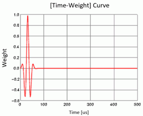
hot/Edge	Electric	Electric Potential	Specify Electric Potential = 1 [V] ☑ Time Dependency Weight is as in the graph below
earth/Edge	Electric	Electric Potential	Specify Electric Potential = 0 [V]

The driving frequency is set to 40 kHz as explained in the analysis condition. Using a spreadsheet, the sine wave of 40 kHz is created, and part of it is used for the [time - weight] graph.

The numerical data created on the spreadsheet can be copied and pasted to the [Time - Weight] table.

Results

The model is analyzed with the timestep manually specified. The results are shown below.

1. Piezoelectric Analysis

Piezoelectric Analysis	1: 4.107499e+04 Hz
Displacement [m]	Z component
0°	Linear

The result fields can be viewed.

At [Results] tab - [Display] - [Solver],select [Piezoelectric Analysis] to see the results of the piezoelectric-resonant analysis.

Of the three vibration modes that were solved, this mode has the largest coupling coefficient. The coupling coefficient can be confirmed in the result table.

The figure below is a contour diagram of Z displacement drawn over the displacement diagram.

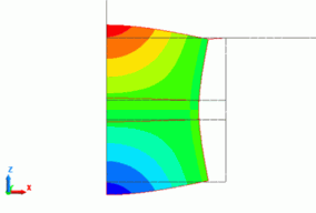Fig 1.

2. Piezoelectric/Time response

Piezoelectric/Time response	24: 4.800000e-05 [s]
Displacement [m]	Z component
	Linear

At [Results] tab - [Display] - [Solver],select [Piezoelectric/Time Response] to see the results of the [Transient Analysis].

Here, you can examine the vibration when the [time - weight] graph is applied. The [time - weight] graph is specified for the boundary condition "hot". Fig. 2(b) is a Z displacement graph that is observed at a point A in Fig. 2(a). The mode is on the horizontal axis.

Fig. 2(a) is a contour diagram at the time indicated by a marker in Fig. 2(b). A contour diagram is drawn over the displacement diagram. The vibration occurs in the mode shown in Fig. 1.

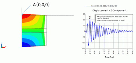
Fig. 2(a) Fig. 2(b)

3. Acoustic Analysis

Acoustic Analysis	82: 1.640000e-04 [s]
Sound Pressure [Pa]	Value
	Linear

At [Results] tab - [Display] - [Solver],select [Acoustic Analysis] to see the results of the acoustic analysis.

The sound pressure distribution is shown in Fig. 3. The sound pressure driven by the piezoelectric material reaches the obstacle placed in the center.

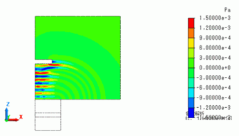
Fig. 3

Fig. 4 is a power graph. In the Result Table, set solver to [Acoustic Analysis], set selection mode to [Show all results summary] , and select [Power] tab. Then press Graph button to draw a graph with time on the horizontal axis and power on the vertical axis.

The power becomes negative at around 300us. It indicates that the waves return after reflection at the obstacle.

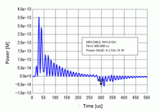
Fig. 4

The sound pressure distribution at 300[us] is shown below. As expected, it is confirmed that the reflected waves return to the piezoelectric material from the obstacle.

Acoustic Analysis	150: 3.0000e-04 [s]
Sound Pressure [Pa]	Value
	Linear

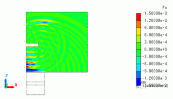
Fig. 5