


|
Home / Examples / Piezoelectric Analysis [Rayleigh] / Example 16: Open Boundary (PML)
Example 16: Open Boundary (PML)
General
-
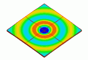
Transverse waves propagating in a piezoelectric substrate are analyzed.
-
The model is surrounded by the open boundary (PML).
-
A quarter model is analyzed.
-
Unless specified in the list below, the default conditions will be applied.
-
Obtain this session's project file. (Right-click and choose 'Save link as')
-
Results will vary depending on Femtet version and the PC environment.
Analysis Space
|
Item |
Settings |
|
Analysis Space |
3D |
|
Model Unit |
mm |
Analysis Conditions
|
Item |
Settings |
|
Solver |
Piezoelectric Analysis [Rayleigh] |
|
Analysis Type |
Harmonic Analysis |
Harmonic Analysis tab and Open Boundary tab are set as follows.
|
Tab |
Setting Item |
Settings |
|
Mesh |
General Mesh Size |
1.0 |
|
Harmonic Analysis |
Sweep Values |
50×103 [Hz] |
|
Sweep Type |
Single Frequency |
|
|
Sweep Setting |
Deselect Fast Sweep. |
|
|
Input |
1.0 [W] |
|
|
Open Boundary |
Type |
PML |
|
PML Thickness |
0.3 [wavelength] |
|
|
Coefficient of PML Damping |
1.0 |
|
|
Wavelength |
0.012 [m] |
[Wavelength] of the open boundary in the above list is the wavelength of elastic wave that is to be absorbed by PML.
This [wavelength] is used only to determine the PML thickness. This value is multiplied by [PML thickness] (unit: wavelength) to determine the thickness for the PML used in the analysis. The value of 0.012 [m] for [Wavelength] in the PML Setting is a reading of the analysis result.
As the wavelength is unknown for the initial analysis, 0.0 [m] is entered for [Wavelength]. By doing so, the PML thickness is determined based on the wavelength of the longitudinal wave which is calculated from the material. The thickness of PML determined in this way tends to be thicker than necessary. The calculation time can be reduced by entering the actual wavelength.
In the Fig. 3(a) below, the peak-to-peak (or bottom-to-bottom) distance of the red line corresponds to the wavelength. It is about 12 mm. Based on this reading, the value is entered for [Wavelength].
-
For your reference, see Open boundary tab and PML in the Technical Note.
Graphical Objects
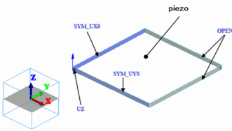
Forced displacement is applied on the center of a large plate. A quarter model is analyzed.
The planes of symmetry are YZ and ZX planes.
Body Attributes and Materials
|
Body Number/Type |
Body Attribute Name |
Material Name |
|
0/Solid |
piezo |
000_P-4 |
(*) Available from the material DB
Boundary Condition
|
Boundary Condition Name/Topology |
Tab |
Boundary Condition Type |
Settings |
|
OPEN/Face |
Mechanical |
Open Boundary |
|
|
UZ/Vertex |
Mechanical |
Displacement |
1.0X10^-3 [m] in Z Direction |
|
SYM_UX0/Face |
Symmetry/Continuity |
Face of Symmetry |
|
|
SYM_UY0/Face |
Symmetry/Continuity |
Face of Symmetry |
|
|
Outer Boundary Condition |
Mechanical |
Free |
|
|
Electric |
Magnetic Wall |
Select on the open boundary tab of the analysis condition setting. |
SYM_UX0 is set with Reflective Symmetry , so it is fixed in X direction.
SYM_UY0 is also set with Reflective Symmetry , so it is fixed in Y direction.
The results of the full model can be viewed with the [Full Model] function.
Results
The contour of displacement in Z direction is shown below. Concentric acoustic waves are propagating outward.
PML is hidden in Fig. 1. It is shown in Fig. 2. The displacements are damped in the PML. The wave is traveling wave.
The animation effectively portrays how the wave travels, making it easily understandable.
To zoom in to the model, [Full Model] is deselected.
The diagram below is shown in the same size of the quarter model.
-
Obtain the animation file. (Save the file before open)
-
Results will vary depending on Femtet version and the PC environment.
To show concentric circles well in the animation, [Gradation contour with color division] is selected on the [Contour tab] of [Graphics Setup] in the Results Window.
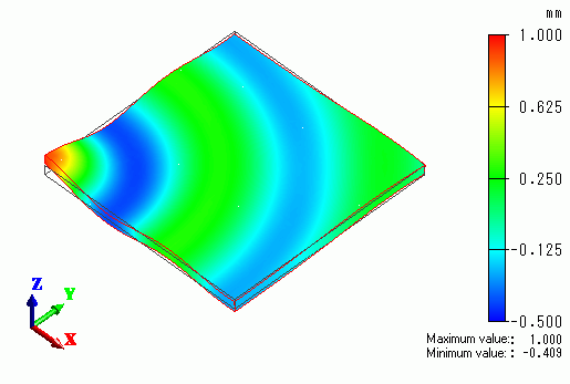
Fig. 1 Z displacement contour
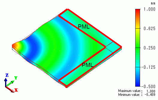
Fig. 2 Z displacement contour (PML is shown)
|
|
|
|
Fig. 3(a) Z displacement phase 0 and absolute |
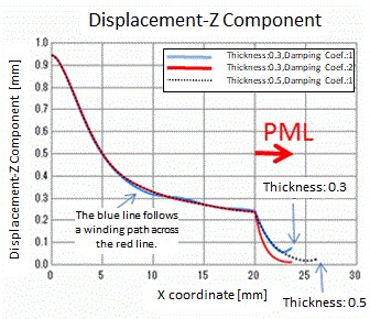
Fig. 3(b) Z displacement absolute Effect of thickness and coefficient of damping |
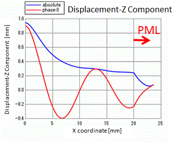
Z component of displacement on the edge area along the X axis is shown in the Fig. 2. The overlapping diagram of phase 0 and absolute is shown in Fig. 3(a).
The absolute is damping rapidly in the PML area.
Fig. 3(b) shows the effect of correcting parameters of PML. The red line is a result of correction of coefficient of damping from 1 to 2.
The black dotted line is a result of thickness correction from 0.3 to 0.5. Except for PML area, red line and black dotted line match and they damp smoothly.
The red line is damping rapidly in the PML area because the coefficient of damping is increased.
The blue line is a result without correction. It slightly deviates from other lines.
It can be estimated that correcting thickness and coefficient of damping contribute to the improvement of the characteristics.
-
For your reference, see Open boundary tab and PML in the Technical Note.