


|
Home / Examples / Coupled Analysis / Thermal-Stress Analysis [Watt/Galileo] / Example 1: Deformation due to the Temperature Gradient #1 - Single Material
Example 1: Deformation due to the Temperature Gradient #1 - Single Material
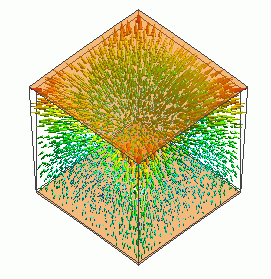
General
-
The deformation due to the temperature gradient on a singe-material cube is analyzed.
-
The temperature distribution is solved in the thermal analysis (Watt) and it can be treated as a reached temperature for a thermal load.
The stress is solved with the thermal load taken into account in the stress analysis (Galileo).
-
The deformation, the displacement distribution, and the stress distribution are solved.
-
Unless specified in the list below, the default conditions will be applied.
-
Obtain this session's project file. (Right-click and choose 'Save link as')
-
Results will vary depending on Femtet version and the PC environment.
Analysis Space
|
Item |
Settings |
|
Analysis Space |
3D |
|
Model Unit |
mm |
Analysis Conditions
Select Thermal analysis and Stress analysis.
|
Item |
Settings |
|
Solver |
Thermal Analysis [Watt] |
|
Thermal-Analysis Type |
Steady-State Analysis |
|
Options |
N/A * |
* [Thermal Load] is selected by default for the thermal-stress coupled analysis.
The Step/Thermal Load tab is set as follows.
|
Tab |
Setting Item |
Settings |
|
Step/Thermal Load * |
Reference Temperature |
0 [deg] |
* The reached temperatures come from the thermal analysis.
Model
The model is a cubic solid body. The material is the polycarbonate. The temperature is fixed at the top and bottom faces.
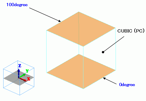
Body Attributes and Materials
|
Body Number/Type |
Body Attribute Name |
Material Name |
|
0/Solid |
CUBIC |
002_Polycarbonate(PC) * |
* Available from the material DB
Boundary Conditions
Thermal analysis is performed based on the boundary conditions below. The resulting temperature distribution is forwarded to stress analysis.
|
Boundary Condition Name/Topology |
Tab |
Boundary Condition Type |
Settings |
|
100degree/Face |
Thermal |
Temperature |
100 [deg] |
|
0degree/Face |
Thermal |
Temperature |
0 [deg] |
Results
The temperature distribution as a result of Watt is shown below.
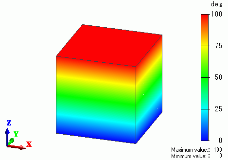
The next figure shows the vectors of displacement as a result of Galileo following Watt.
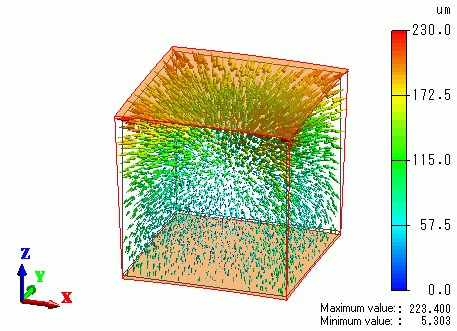
The expansion is larger at the top of the model.