


|
Home / Examples / Coupled Analysis / Thermal-Stress Analysis [Watt/Galileo] / Example 7: Model with Reflective Symmetry
Example 7: Model with Reflective Symmetry
General
-
A quarter model of the example 2 is analyzed with reflective symmetry applied.
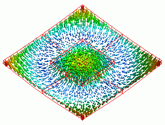
The figure above is obtained with [Full Model].
-
The reflective symmetry is used as boundary condition.
-
The temperature distribution is calculated with the thermal solver (Watt).
With the temperature distribution set to the reached temperature in the thermal load, the stress is calculated with the stress solver (Galileo)
-
The deformation, the displacement and the stress are solved.
-
Unless specified in the list below, the default conditions will be applied.
-
Obtain this session's project file. (Right-click and choose 'Save link as')
-
Results will vary depending on Femtet version and the PC environment.
Analysis Space
|
Item |
Settings |
|
Analysis Space |
3D |
|
Model Unit |
mm |
Analysis Conditions
Select Thermal analysis and Stress analysis.
|
Item |
Settings |
|
Solver |
Thermal Analysis [Watt] |
|
Thermal-Analysis Type |
Steady-State Analysis |
|
Options |
N/A * |
* [Thermal Load] is selected by default for the thermal-stress coupled analysis.
The Step/Thermal Load tab is set as follows.
|
Tab |
Setting Item |
Settings |
|
Step/Thermal Load * |
Reference Temperature |
25 [deg] |
* The reached temperatures come from the thermal analysis.
Model
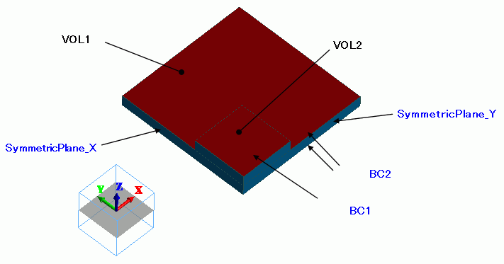
This is a quarter model of example 2.
The planes of symmetry are YX and ZX planes.
Body Attributes and Materials
|
Body Number/Type |
Body Attribute Name |
Material Name |
|
0/Solid |
VOL1 |
006_Glass_epoxy * |
|
1/Solid |
VOL2 |
001_Alumina * |
* Available from the material DB
The heat quantity of VOL2 is set up as follows.
enter 0.25 [W] which is a quarter value of the original model.
|
Body Attribute Name |
Tab |
Settings |
|
VOL2 |
Heat Quantity |
0.25 [W] |
Boundary Conditions
Set reflective symmetry on the applicable topologies.
|
Boundary Condition Name/Topology |
Tab |
Boundary Condition Type |
Settings |
|
BC1/Face |
Thermal |
Heat Transfer/Convection |
Coefficient of Heat Transfer: 17.26 [W/m2/deg] Room Temperature: 25 [deg] |
|
BC2/Face |
Thermal |
Heat Transfer/Convection |
Coefficient of Heat Transfer: 27.3 [W/m2/deg] Room Temperature: 25 [deg] |
|
SymmetricPlane_X/Face |
Symmetry/Continuity |
Symmetry |
Reflective |
|
SymmetricPlane_Y/Face |
Symmetry/Continuity |
Symmetry |
Reflective |
The coefficient of heat transfer for the forced convection is calculated as follows.
h = 3.86 x (V/L)0.5 x C [W/m2/deg]
where
Air flow V=1 [m/s]
Top and Bottom Faces of Substrate (VOL1): Typical Length L=0.05, C=1 -> h=17.26
Top Face of Heat Source (VOL2): Typical Length L=0.02, L'=0.015, C=1 * -> h=27.3
*
The thickness (d) of the speed boundary layer at the edges of the heat source is given by
δ = 0.0182x(L’/V)0.5 = 2.3 [mm]
This is close enough to the thickness of heat source, so we set C=1.
|
Boundary Condition Name/Topology |
Tab |
Boundary Condition Type |
Settings |
|
BC1/Face |
Thermal |
Heat Transfer/Ambient Radiation |
Coefficient of Heat Transfer: 17.26 [W/m2/deg] Room Temperature: 25 [deg] |
|
BC2/Face |
Thermal |
Heat Transfer/Ambient Radiation |
Coefficient of Heat Transfer: 27.3 [W/m2/deg] Room Temperature: 25 [deg] |
Thermal analysis is performed based on the boundary conditions below. The resulting temperature distribution is forwarded to stress analysis.
Results
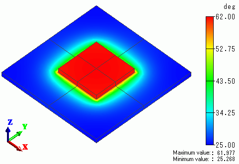
The temperature distribution as a result of Watt is shown below.
The next figure shows the vectors of displacement as a result of Galileo following Watt.
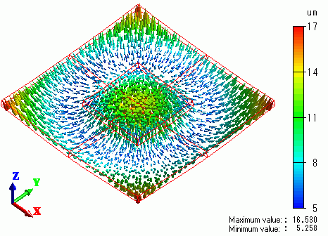
They are quite similar to the results of example 2.