|
Home / Show Results / Visualization Tool for the Heat Path
Visualization Tool for the Heat Path
1. Overview
It is difficult to grasp the rough idea of the heat flow by Femtet's display function alone.
Temperature contour: The heat path cannot be identified because the heat flow is not visualized.
Heat flux vectors: The flow direction is visible but the actual heat flow rate is not known.
Numerical display of heat balance, heat flow rate, thermal resistance: In-depth understanding of the data is required to grasp the heat flow.
To address the problems above, Excel tool is prepared to visualize the heat flow.
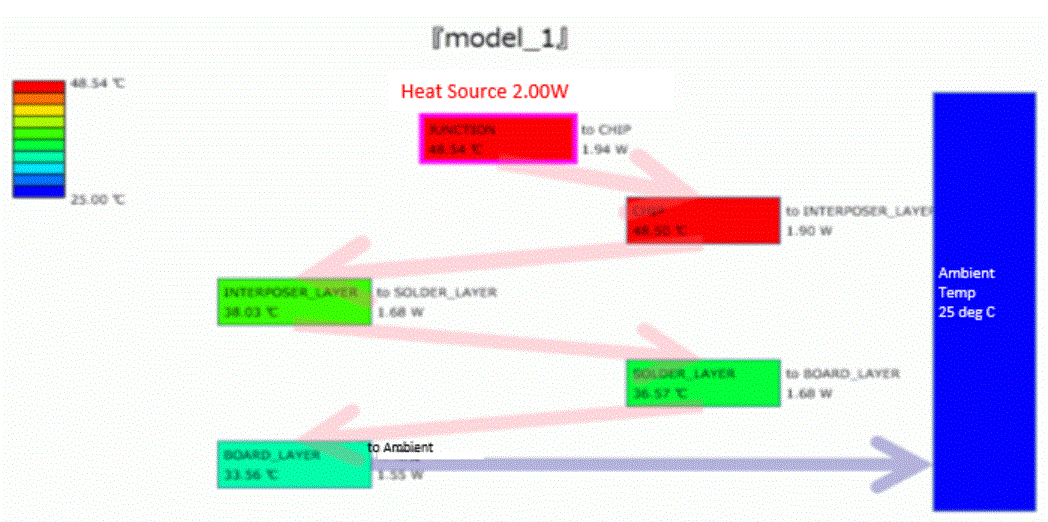
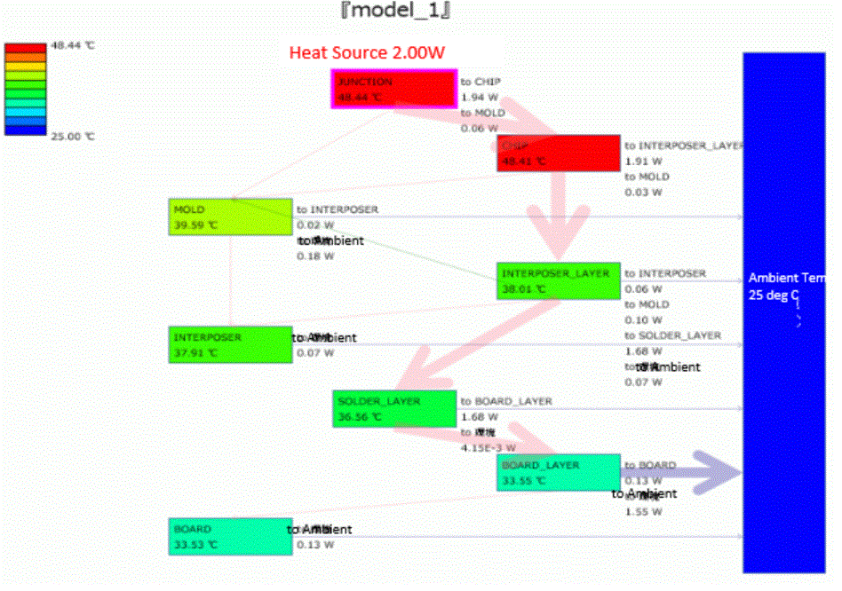
Example: Analysis model 1 of Example 22: Junction Thermal Resistance of Semiconductor Package.
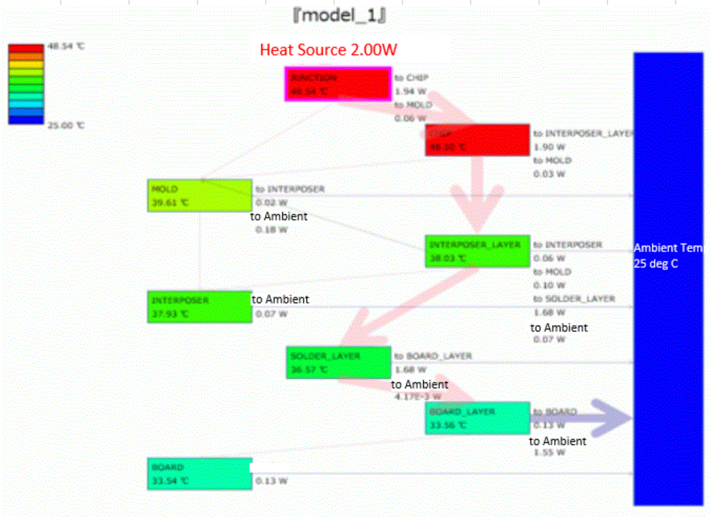
The heat of JUNCTION (heat source) is released to the environment.
It reaches the environment through chip, mold, interposer, solder, and substrate.
The thickness of the arrow indicates the magnitude of the heat flow rate. Its thickness gives you a rough idea of the heat flow.
The heat flows mainly through the path of JUNCTION (heat source) -> interposer -> solder -> substrate -> environment.
2. Features of the Tool
- The tool is available for the steady-state analysis only.
- The heat transfer between the body attributes or boundary conditions can be visualized.
- Each body attribute or boundary condition is displayed by a box called node. The heat transfer is indicated by an arrow.
- On the right side of the box shows the destination of the heat transfer and the heat flow.
- The node with higher temperature is placed in the upper side of the chart and the node with lower temperature is placed in the lower side of the chart. (The heat transfers from the upper side to the lower side of the chart.)
- The magnitude of the heat flow is represented by the thickness of the arrow.
- The ambient temperature such as the natural convection boundary condition is shown at the right side of the box.
- The heat transfer to the boundary having no ambient temperature is shown on the left side of the box.
- The heat quantity is displayed at the top of the box. The endothermic is shown at the bottom of the box.
- In the [Thermal Resistance] sheet, the thermal resistance is displayed instead of the heat flow.
(As the thermal resistance is calculated with the average temperature difference, the value may be unnatural in some cases.)
3. Download
Click the link below to download the tool.
ThermalCascadeViewer_2025_0.xlsm
4. How to Use
- In the steady-state analysis of the thermal solver, [analysis model name_heatflow.csv] and [analysis model name_heatflow_el.csv] are created in the [project file name.results] folder. (Note 1)
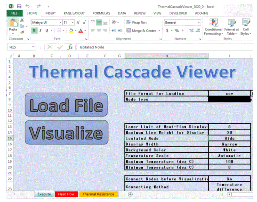
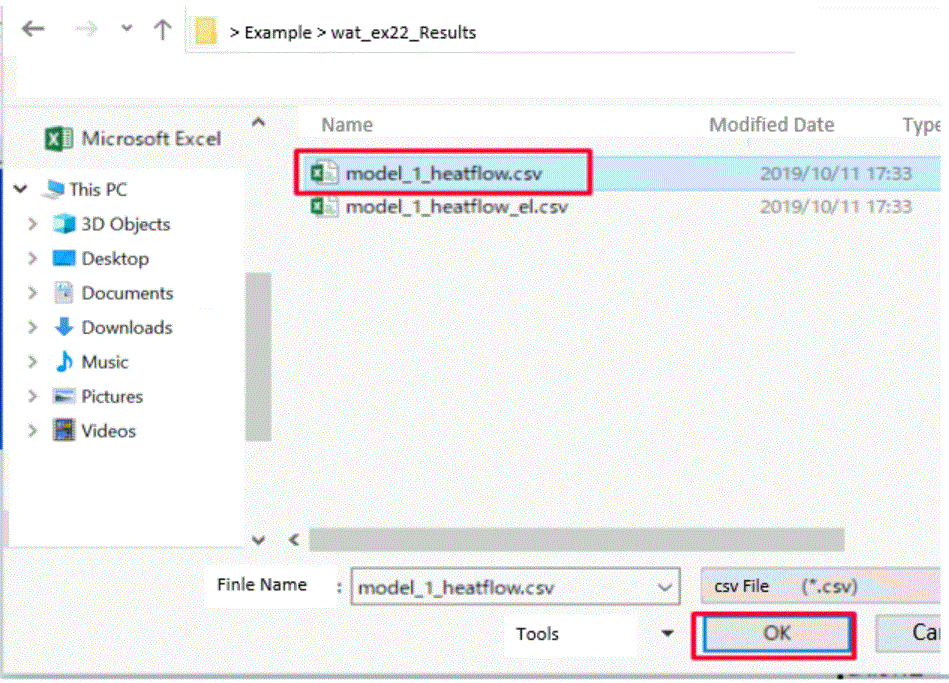
- Click  of the "Execute" sheet of Excel to load a file. Select either [analysis model name_heatflow.csv] or [analysis model name_heatflow_el.csv]. (Note 2)
- The heat flow is displayed on the "Heat Flow" sheet of Excel. The numerical values converted to the thermal resistance are displayed on the "Thermal Resistance" sheet.
- To change the settings, click  to redraw after modifying the settings.
(Note 1)
There may be a case where [analysis model name_heatflow.csv] and [analysis model name_heatflow_el.csv] are not found if parametric analysis is performed.
They can be loaded from [analysis model name.pdt] by selecting pdt format.
To do so, enable the macro function.
Go to [Macro Help Home] > [Preparation for Macro Operation] for the details.
(Note 2)
If [analysis model name_heatflow.csv] is selected, body attribute is selected as a node type for display.
If [analysis model name_heatflow_el.csv] is selected, boundary condition is selected as a node type for display.
Options for Loading
|
|
Options |
Notes |
|
File Format for Loading |
csv / pdt |
Selects the file type for loading. Usually, csv is selected. Refer to Note 1 above. |
|
Node Type |
Body Attribute / Boundary Condition |
<When csv is selected> Selection is not required. The node type is determined by selecting the file type ( [analysis model name_heatflow.csv] or [analysis model name_heatflow_el.csv] ) <Only when pdt is selected> - Body attribute - Boundary condition The selection depends on whether the focus of your interest is the heat flow between the body attributes or the heat transfer to or from the boundary condition. |
Options for Display
|
|
Options |
Notes |
|
Lower Limit of Heat-Flow Display [W] |
Numerical Entry |
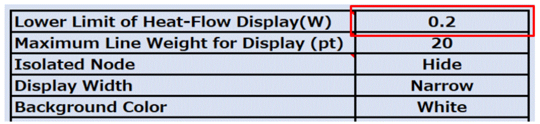
Hides the heat flows smaller than the specified lower limit. |
|
Maximum Line Weight for Display [pt] |
Numerical Entry |
|
|
Isolated Node |
Show / Hide |
Controls show/hide of the nodes that have no inflow or outflow of heat. |
|
Display Width |
Narrow / Wide |
Adjusts the spacing between the horizontally-placed nodes. |
|
Background Color |
White / Gray |
Sets the background color. |
|
Temperature Scale |
Automatic / Manual |
Controls automatic/manual setting of the maximum and minimum values for the temperature scale (color scale). |
|
Maximum Temperature (deg C) |
Numerical Entry |
Sets the maximum value of the temperature scale. |
|
Minimum Temperature (deg C) |
Numerical Entry |
Sets the minimum value of the temperature scale. |
|
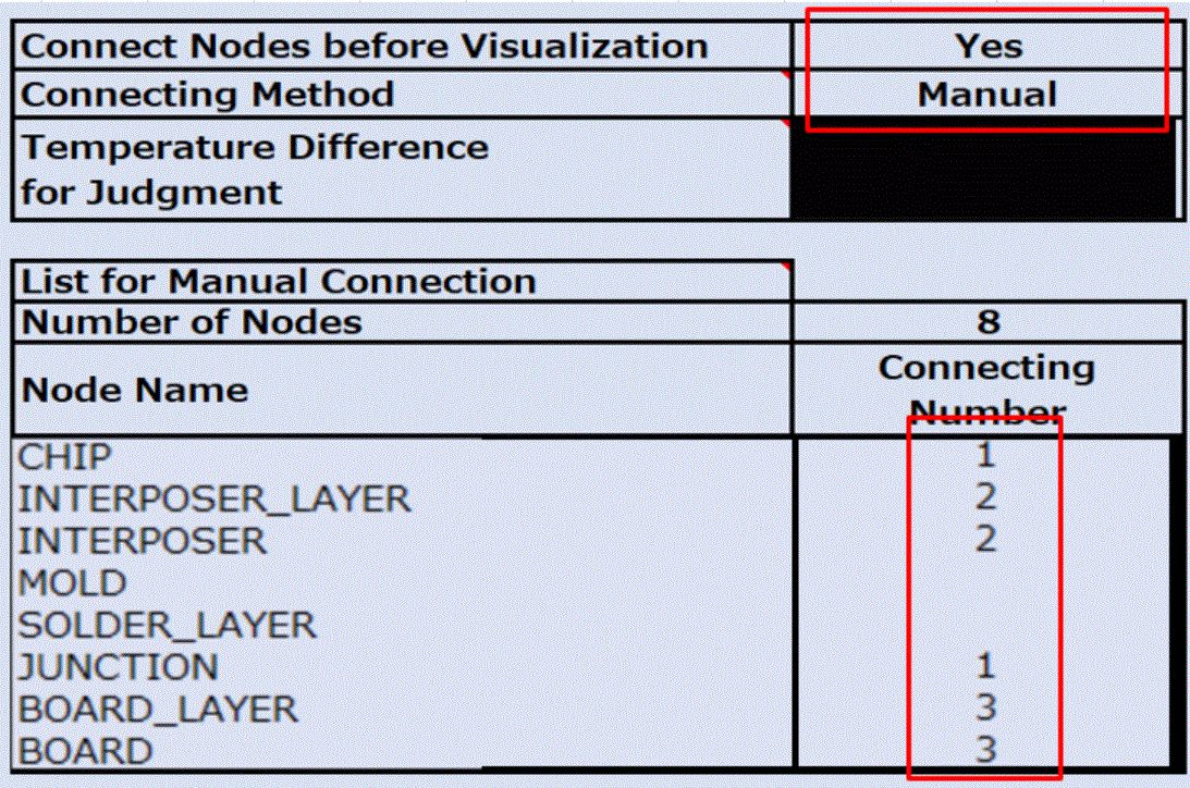
Connect Nodes before Visualization |
Yes / No |
Connects multiple nodes. |
|
Connecting Method |
Temperature Difference / Manual |
Specifies the connecting method. |
|
Temperature Difference for Judgment (deg C) |
Numerical Entry |
Connects the adjacent nodes if the average temperature difference is less than or equal to this value. |
|
List for Manual Connection |
Numerical Entry |
Assigns the connecting number for each node. The nodes having the same connecting number are connected. |
5. Example
|
1. The thermal analysis is performed. |
|
|
2. Open a ThermalCascadeViewer file. |
|
|
3. File Format for Loading: Confirm csv is selected, and click |
|
|
4. To select a file, |
|
|
5. Visualization is executed and the results will be displayed on the [Heat Flow] sheet. |
|
|
6. Enter 0.2[W] in the Lower Limit of Heat-Flow Display so as to show the governing heat flows only. |
|
|
7. Click |
|
|
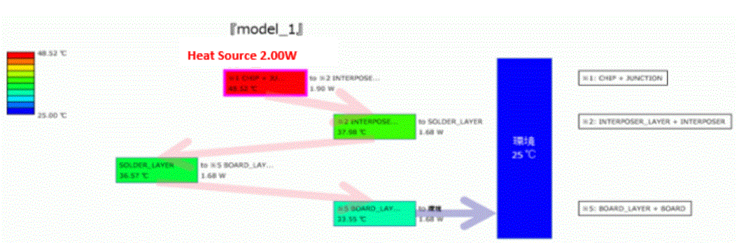
8. Connect the related body attributes for better visibility. |
|
|
9. Click |
|