

Macro Samples
This section introduces examples using macros.
Femtet can be operated using Excel VBA and Python macros.
For the initial settings required to use macros, please refer to the following page.

-
Example 48
Restart analysis with repeated heating on and off
Techniques Used in the Example
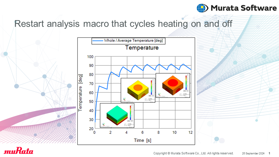
This is a sample macro for a restart analysis in which the specified boundary conditions in a transient heat transfer analysis are alternately switched between the temperature boundary and the convection boundary, and heating and cooling are repeated for a specified time.
The time setting for heating and cooling and the temperature setting for heating can be set from the Excel worksheet.
The program code for macro control is very simple because it controls the macro of the project file created in advance.Simulation Image
-
Example 42
Geometry Creation Macro by Loft on Curve
Techniques Used in the Example
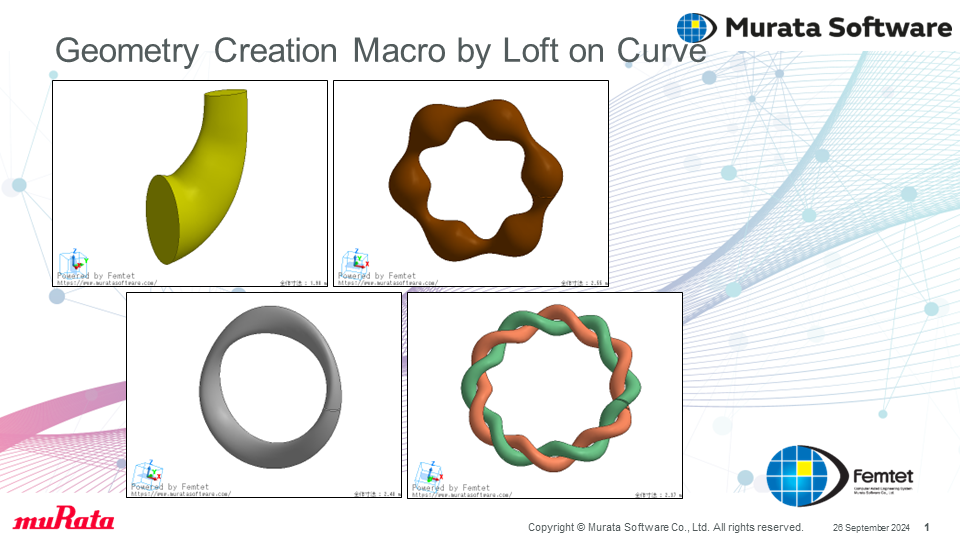
The Loft function allows you to create a solid shape by smoothly connecting different sheet bodies.
This macro shows how to create a complex shape that is difficult to create by GUI by placing an ellipse (or circle) with a slightly different shape and angle on a curve and lofting it.Examples of specific shapes include Mobius rings, constricted rings, and twisted pair rings.
Simulation Image
-
Example 40
Radiation analysis with moving heat source
Techniques Used in the Example
Macro sample for radiation analysis with moving heat source is shown.
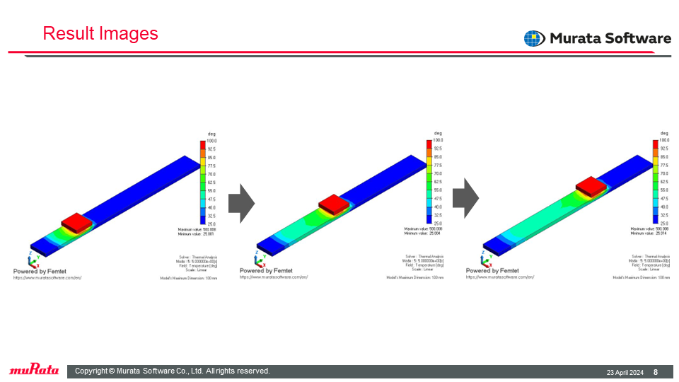
The macro automates the process of moving the heat source body through a variable and repeating the transient analysis with the previous final temperature imported as the initial temperature in the results import.
The process of saving the result file for each variable condition and saving the image of the temperature distribution of all modes in each result file is also automated by the macro.Simulation Image
-
Example 39
Restart analysis to change heat source value according to monitor temperature
Techniques Used in the Example
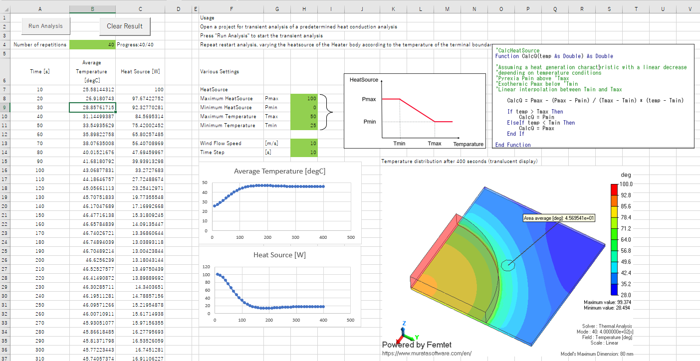
This example repeats the restart analysis of the heat conduction transient analysis by changing the heatsource value of the heating body according to the monitor temperature of the measurement terminal boundary.
The process of changing the heating condition of the heating body according to the temperature condition of the measurement terminal boundary cannot be simulated by the temperature dependence of the heating density, so it is necessary to use a macro.
In the sample condition, you can see how the heating value decreases with increasing temperature and converges to certain temperature and heating conditions.Simulation Image
-
Example 38
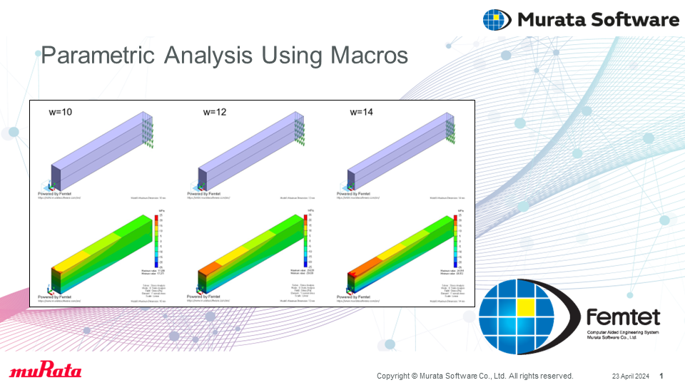
Parametric analysis using macros
Techniques Used in the Example
An example of a macro (VBA) that automatically opens the project file for the variable Femtet,
repeats the analysis, changing the variables according to the set conditions
and saves model and result diagrams.Simulation Image
-
Example 37
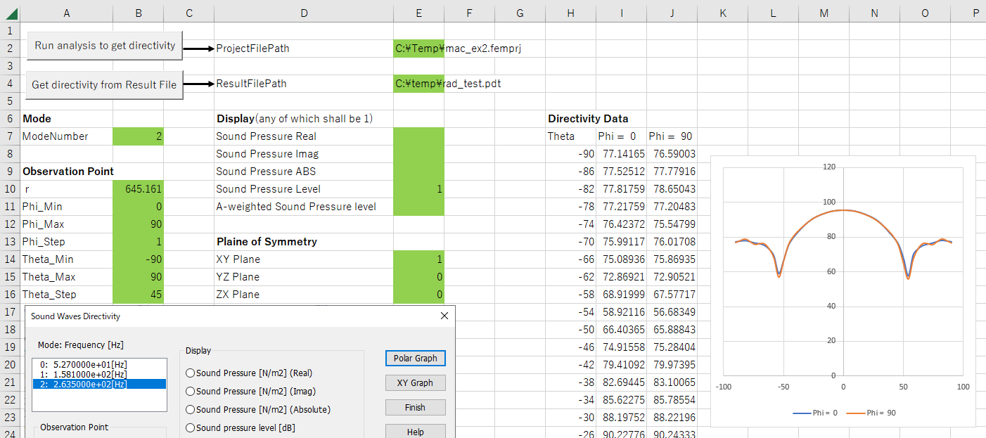
Acquisition of sound pressure directivity data for sound analysis
Acquisition of sound pressure directivity data for sound analysis
1 You can execute the specified project file to obtain directivity.
2 The specified result file can be opened to obtain directivity.The directional result is the result of swinging theta and phi into the array variable, which is stored serially.
You must understand its internal array before retrieving it.
The SamplingResult function in this macro shows an example of this process.Simulation Image
-
Example 35
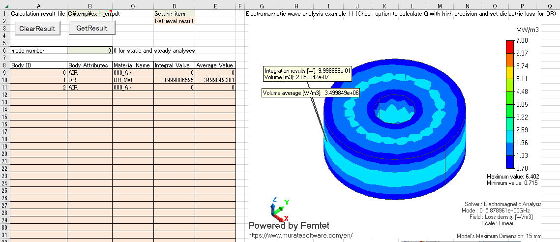
Get integrated and averaged potentials per body
Techniques Used in the Example
Macro to get the integral and average values of the potentials per body.
Support for getting results in all bodies (single mode specification) or all modes (single body specification).
It corresponds to obtaining integral and average values of three potentials: temperature for heat conduction analysis, loss density for electromagnetic wave analysis, and elastic equivalent strain for stress analysis.
If you want to obtain the integral and average values of other potentials, you can modify the functionality by editing the SetResultField and SetResultMode functions in the standard module.
*Only 3D models are supported.Simulation Image
-
Example 32
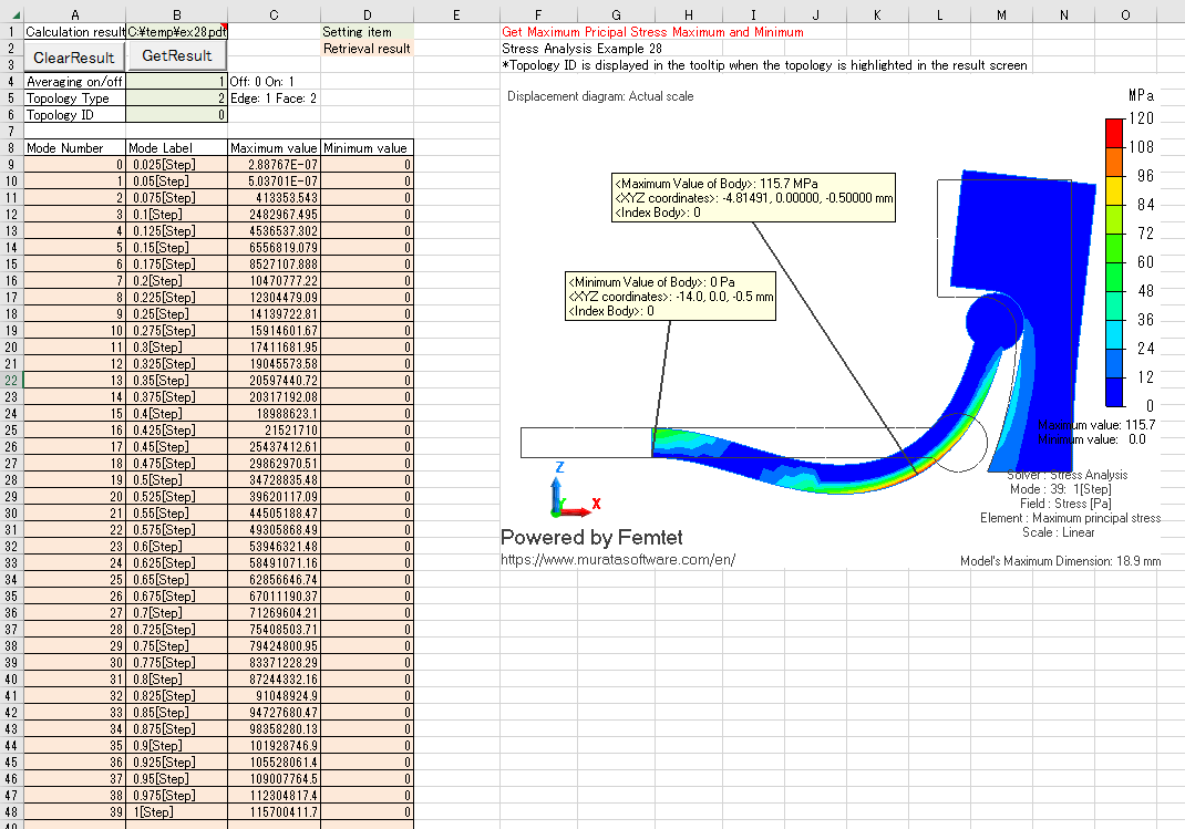
Get the maximum value and minimum value for a given topology (Edge, Face)
Techniques Used in the Example
A macro that returns the maximum and minimum values of a nodal result in a previously specified topology (edge or face).
Support for retrieving results in multiple topologies (single mode specification) or all modes (single topology specification).
Corresponds to obtaining three results: temperature for heat conduction analysis, magnitude of field vector for electric field analysis, and maximum principal stress for stress analysis.
To obtain the maximum and minimum values of other node results, you can modify the functions SetResultField, SetResultMode, and GetResultNode in the standard module.For fields that are discontinuous at element boundaries, such as stresses and electric fields, the maximum value and minimum value change depending on the averaging on/off setting of the drawing settings, but also correspond to the averaging on/off setting.
Techniques Used in the Example
-
Example 30
Calculation of Area and Volume of Portion having temperatures in the specified range
Techniques Used in the Example
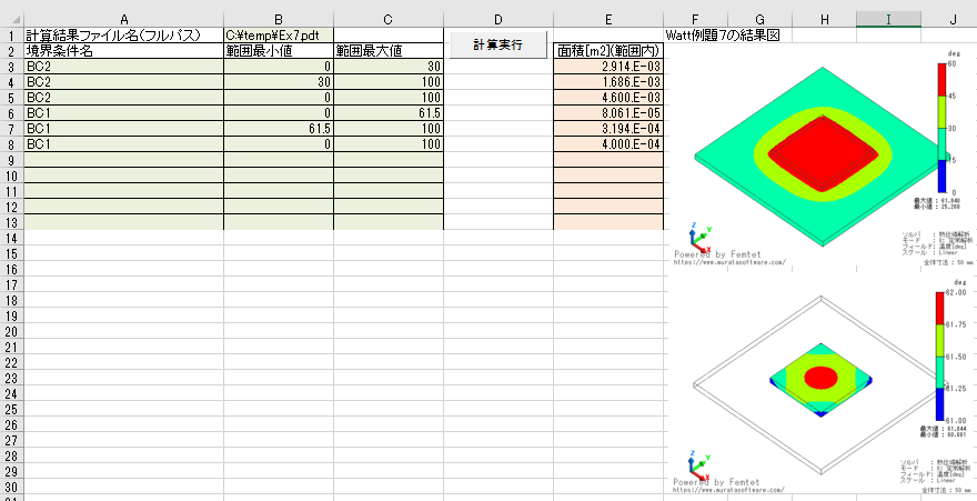
The macro can open the result file of the thermal solver and calculate the area and volume of the portion having temperatures in the specified range.
Specifies the boundary condition name or FaceID for area calculations or the body attribute name or BodyID for volume calculations.
Conditional branch processes check the temperature at an integral point.Simulation Image
-
Example 29
Save Results Image File Automatically (Thermal Analysis)
Techniques Used in the Example
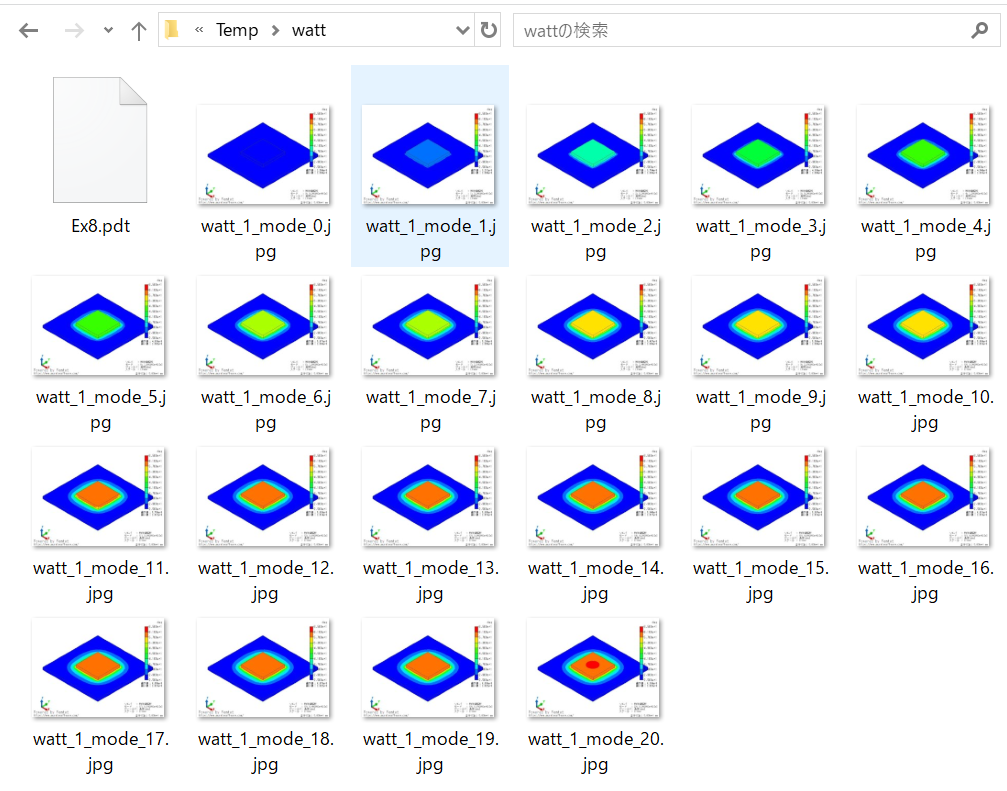
You can automatically save temperature distribution diagrams of the specified results file.
In the case of different modes in the transient analysis, you can automatically save all the diagrams.
You can set the maximum and minimum values for the view vector, image size, and temperature color scale.Simulation Image
-
Example 26
Maximum Principal Stress and Von Mises Equivalent Stress
Techniques Used in the Example
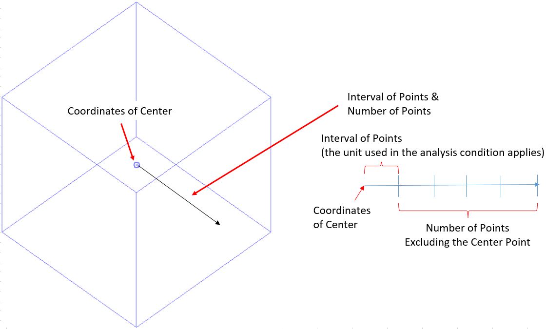
You can extract the maximum principal stress and von Mises equivalent stress in the 3D lattice.
You can learn how to extract the results of your wish automatically from the calculation.Simulation Image
-
Example 25
Access Log Checking
Techniques Used in the Example
You can check the login time.
Simulation Image

-
Example 24
Convert Nastran format to STL format with deformed shapes.
Techniques Used in the Example
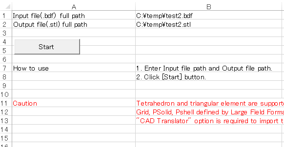
This macro converts nastran format file that includes mesh data with displacements to STL format file.
It is possible to import the output STL format file into other CAD software.Simulation Image
-
Example 23
Free Curves
Techniques Used in the Example
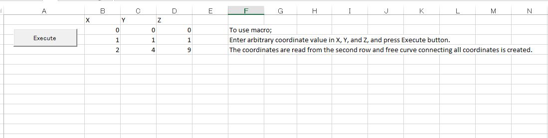
You can create the free curves connecting all coordinates by reading the entered coordinates.
By entering the coordinates given by the parabola equation, a parabola body can be created.Simulation Image
-
Example 22
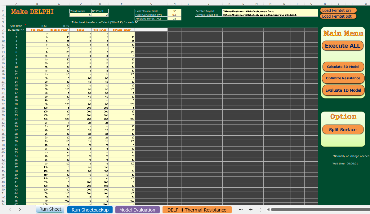
Deriving a DELPHI Model (1D Thermal Analysis Model) Using the Femtet Macro
Techniques Used in the Example
This macro automates the process of deriving a DELPHI model (1D thermal analysis model) from a Femtet model.
Simulation Image
-
Example 21
Magnetic Flux Integration by Integrand
Techniques Used in the Example
・You can integrate the specified faces of the multiple results.
You can learn how to integrate the arbitrary faces with the integrand.Simulation Image
-
Example 20
Damping Calculation of Sound Waves for Acoustic Analysis
Techniques Used in the Example
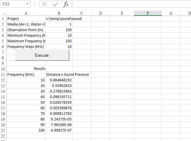
You can calculate the damping of sound waves when they propagate in the lossy media.
You can learn how to set the complex sound speed and obtain the results of sound pressure.Simulation Image
-
Example 19
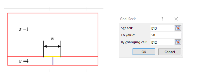
Optimization by Goal Seek
Techniques Used in the Example
You can calculate the electrode width so as to set the characteristic impedance of microstrip line to 50 ohms.
You can learn how to optimize the characteristic impedance and obtain the results.Simulation Image
-
Example 18
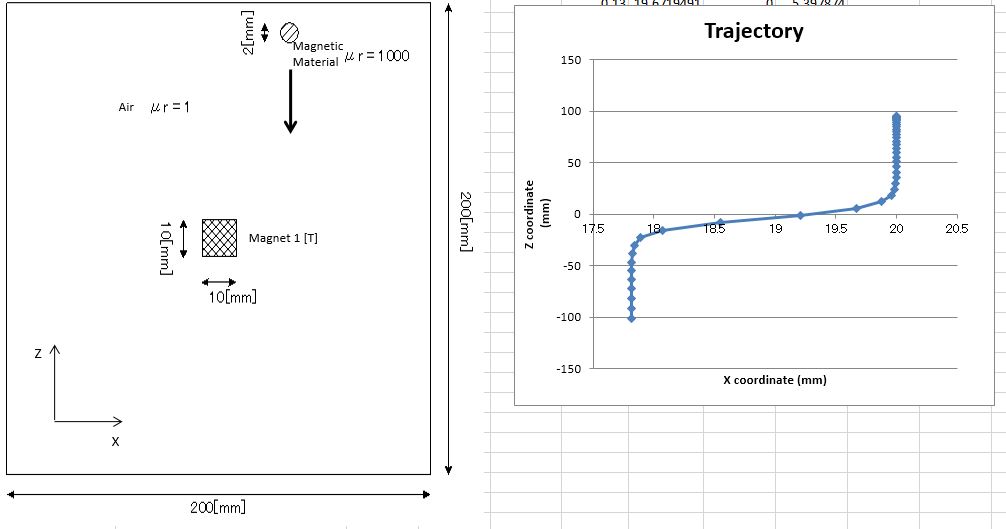
Trajectory Calculation of Free-falling Magnetic Object for Magnetic Analysis
Techniques Used in the Example
You can calculate the trajectory of a free-falling magnetic object.
You can learn how to obtain the electromagnetic force from the results and graph the results.Simulation Image
-
Example 17
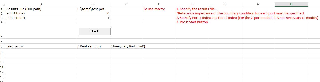
Impedance Calculation between Ports for Electromagnetic Analysis
Techniques Used in the Example
You can calculate the impedance between the two ports using the the electromagnetic analysis results.
You can learn how to convert the S-parameters to the Z-parameters.Simulation Image
-
Example 16
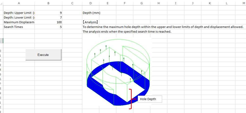
Recalculation by the Feedback of the Results for Stress Analysis
Techniques Used in the Example
You can recalculate by modifying the analysis conditions.
You can learn how to feedback the results to analysis model and analysis conditions.Simulation Image
-
Example 15
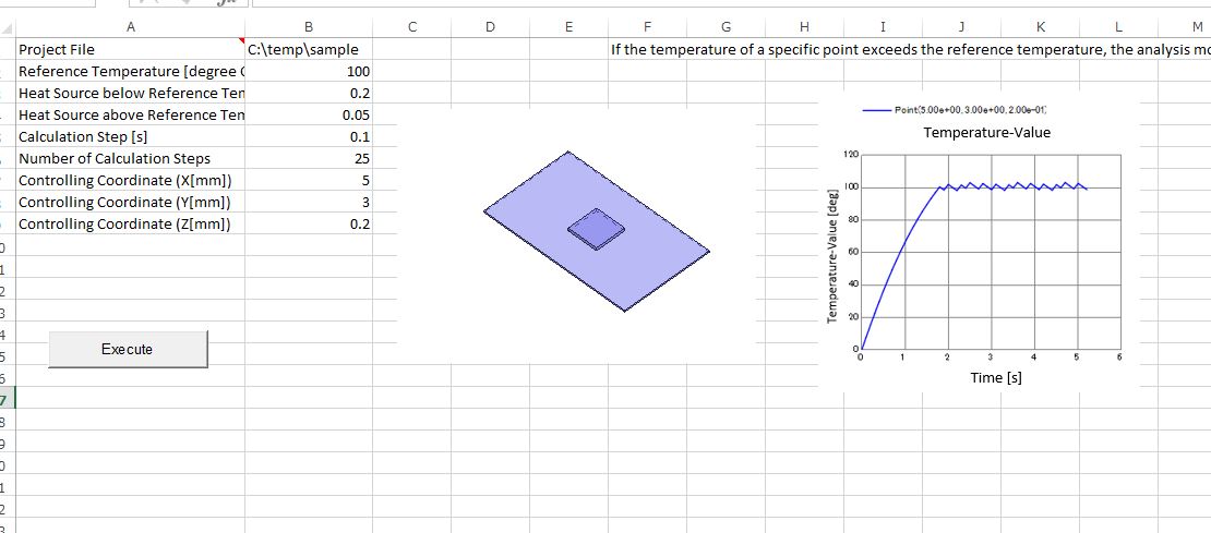
Recalculation by the Feedback of the Results for Thermal Analysis
Techniques Used in the Example
You can recalculate by modifying the analysis conditions.
You can learn how to feedback the results to analysis model and analysis conditions.Simulation Image
-
Example 14
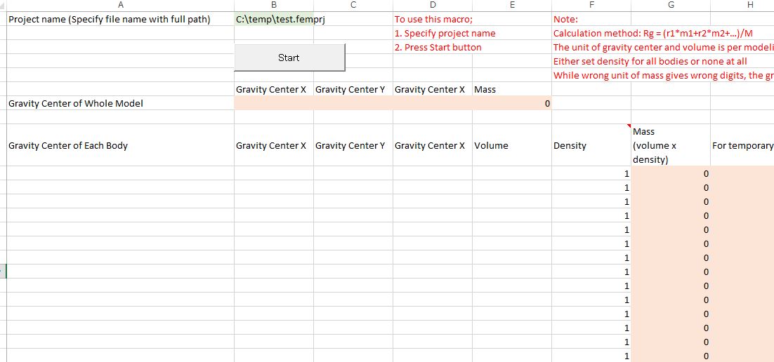
Gravity Center of Whole Model
Techniques Used in the Example
You can calculate the gravity center of the whole model by getting gravity center, volume, and density of the body.
You can learn how to obtain the body’s properties such as gravity center and volume.Simulation Image
-
Example 13
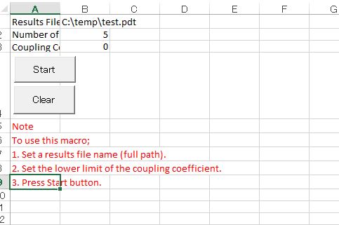
Save Specified Results Window for Piezoelectric Analysis
Techniques Used in the Example
You can specify and save the results of all modes as an image.
Also, you can filter the modes by specifying the coupling coefficient to remove the unwanted modes.Simulation Image
-
Example 12
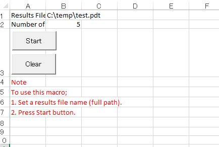
Save Specified Results Window for Stress Analysis
Techniques Used in the Example
You can specify and save the results of all modes as an image.
Simulation Image
-
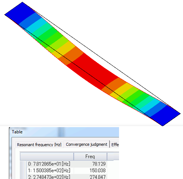
Example 10
Resonant Analysis with Initial Stress Taken into Account
Techniques Used in the Example
CAD data is imported for static analysis.
Its results are used as an initial stress in the resonant analysis.
You can learn how to import CAD data, duplicate a project, and extract results automatically.Simulation Image
-
Example 9
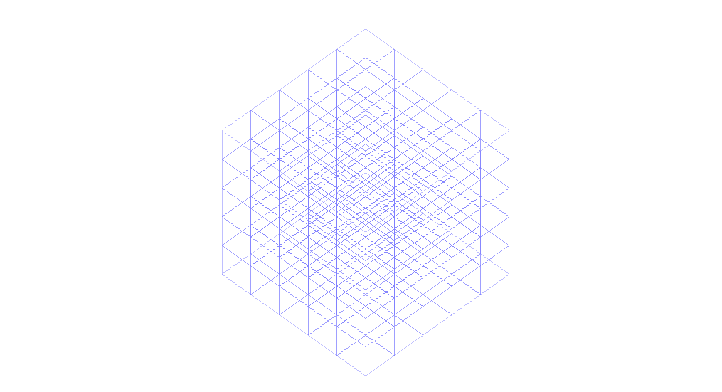
Results in 3D Grids
Techniques Used in the Example
The results are saved in 3d grids.
You can learn how to extract the results of your wish from the calculation results.Simulation Image
-
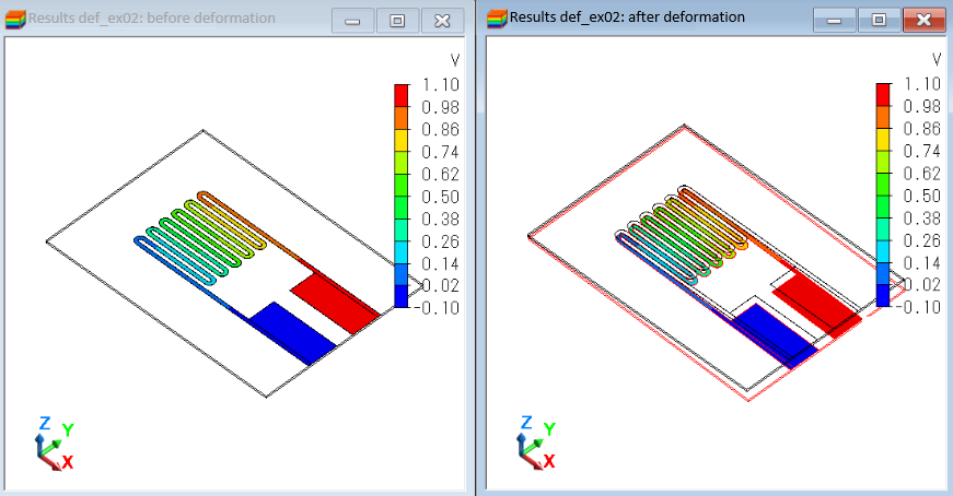
Example 8
Execute Analysis with Reference to the Existing Meshes
Techniques Used in the Example
You can learn how to execute a specific processing for multiple files.
Simulation Image
-
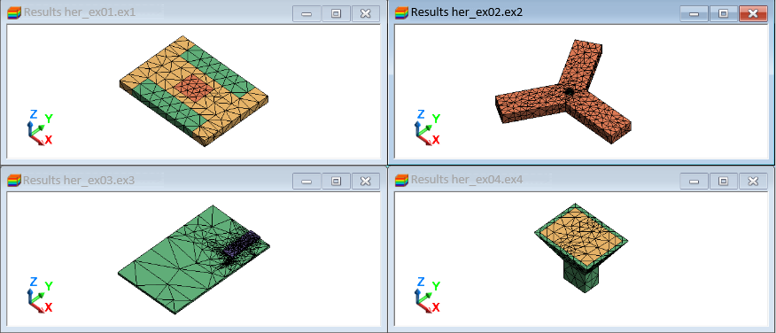
Example 7
Generate Only Meshes for Multiple Projects
Techniques Used in the Example
You can learn how to execute a specific processing for multiple files.
Simulation Image
-
Example 6
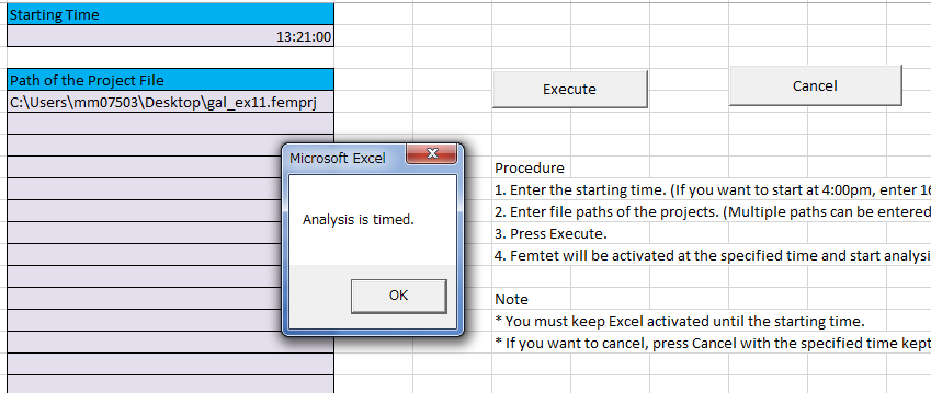
Timed Analysis
Techniques Used in the Example
Analysis is executed at the specified time.
You can learn how to control the processing with OnTime method of ExcelVBA.Simulation Image
-
Example 5
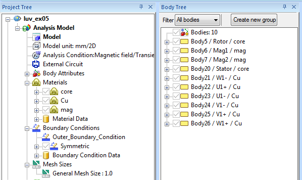
Listing of Material Property Names
Techniques Used in the Example
Material property names in the specified project file are extracted.
You can learn how to extract the information of your wish.Simulation Image
-
Example 4
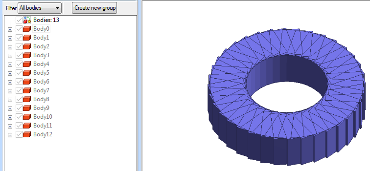
Automatic Assignment of Body Attribute Name
Techniques Used in the Example
A body attribute name is given automatically to the body in the specified project.
You can learn how to edit the multiple bodies collectively.Simulation Image
-
Example 3
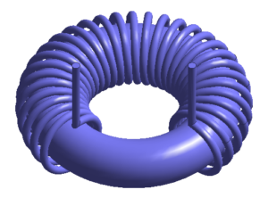
Toroidal Coil (based on Example 7 of Macro Help)
Toroidal Coil (based on Example 7 of Macro Help)
The location of the end of turns of the coil can be specified. A coil of helical/spiral prism can be created.
You can learn how to create a complicated form automatically.Simulation Image
-
Example 2
Save the Results Window of All Modes
Techniques Used in the Example
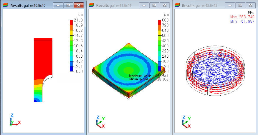
You can learn how to create an analysis model, set conditions, execute analysis, and extract the results with macro.
Techniques Used in the Example
-
Example 1
DXF File Import
Techniques Used in the Example
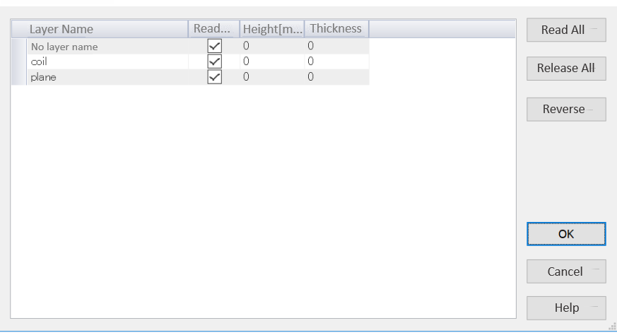
A project file is automatically created with an imported DXF file.
If multiple DXF files are specified, multiple projects are created for each DXF file.
You can learn how to manage files with macro.Simulation Image
Brochure Request & Free Trial
-
Download materials that give you a quick overview of basic features, how to use Femtet, Cases, and more.

-
Apply for Seminars Here

-
Apply Here for a Free Trial
