
General
Home / Examples / Coupled Analysis / Fluid-Thermal Analysis [Bernoulli/Watt] / Example 16: Thermal-Fluid Analysis of Porous Medium
The hot fluid flows into the porous medium which includes many aluminum particles. The flow and the heat are analyzed.
The temperature distribution and the heat flux vectors are solved.
Unless specified in the list below, the default conditions are applied.
Results will vary depending on Femtet version and the PC environment.
Item |
Settings |
Analysis Space |
3D |
Model Unit |
mm |
Item |
Settings |
Solver |
Fluid Analysis [Bernoulli] Thermal Analysis [Watt] |
Analysis Type |
Fluid Analysis: Steady-state Analysis Thermal Analysis: Transient analysis |
Laminar Flow/Turbulent Flow |
Select Turbulent Flow |
Meshing Setup |
General Mesh Size: 10 [mm] |
The setting on the transient analysis tab are as follows. The total calculation steps is 200. The timestep is 0.1 [s].
Therefore, the temperature distributions for 200 [s] following an initial temperature of 25 deg are analyzed.
Tab |
Setting Item |
Setting |
||||||||
Transient Analysis |
Table |
|
||||||||
Initial Temperature |
Use ambient temperature (25 [deg]) |
The cylinder is a solid with its center part having larger diameter. The material of air (000_Air) is defined.
The body attribute of the center part of the body is a porous domain.

Body Number/Type |
Body Attribute Name |
Material Name |
2/Solid |
Porous |
000_Air |
5/Solid |
Pipe |
000_Air |
6/Solid |
Pipe |
000_Air |
* Available from the material DB
The porous part is set on the fluid tab as follows medium.
Body Attribute Name |
Tab |
Settings |
Porous |
Fluid |
Fluid Body Type: Porous Medium Velocity Dependency: Calculate from porosity Porosity: 0.39 Particle Diameter: 10 [mm] Shape Factor: 1.0 Material of Solid: [001_Al]
|
Boundary Condition Name/Topology |
Tab |
Boundary Condition Type |
Settings |
Inlet/Face |
Fluid-Thermal |
Inlet |
Specify flow velocity Flow Velocity: 10 [m/s] Inflow Temperature: Direct Entry, 100[ deg] |
Outlet/Face |
Fluid-Thermal |
Outlet |
Natural Outflow |
By switching the solver from thermal to fluid, the results related to the fluid analysis such as flow velocity and pressure are obtained.
The velocity vectors on the cross section at y=0 are shown.
The averaged flow velocity is displayed for the inside of the porous part. (The velocity in the porous part is at its highest value according to the porosity)

Below is the plotting of the flow velocity from the coordinates (0,0,0) to the coordinates (500,0,0).
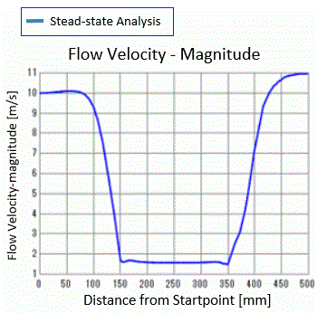
The averaged flow velocity inside of the porous part is about 1.58 [m/s].
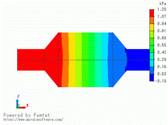
Below is the pressure (static pressure) distribution.
The pressure in the porous part shows a large drop in the porous portion toward the outlet.
If [Calculate from Porosity] is selected in the setting, the coefficient of porous is obtained by the Ergun equation.
The calculation log shows the details.
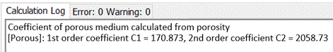
With the averaged flow velocity of 1.58 [m/s] in the porous part and the porous part’s length of 200 [mm], the pressure loss in the porous part can be roughly calculated as follows.
Pressure loss ΔP = (170.873 * 1.58 + 2058.73 * 1.58 * 1.58 ) * 0.2 = 1094 [Pa]
Pressure drop in the pressure distribution matches very well.
Now, let’s switch the solver type to thermal analysis from fluid analysis to examine the thermal analysis results.
The results at 0.1 [s], 5 [s], and 20 [s] are shown below. The maximum and minimum values of the contour diagram are 100 [deg] and 20 [deg], respectively.
The temperature at the inlet rises to 100 [deg] over the time as short as 0.1 [s].
The heat spreads through the inside of the porous part over a long period of time.
That is due to the fact that the specific heat and the density of aluminum are much larger than those of air.
0.1 [s] 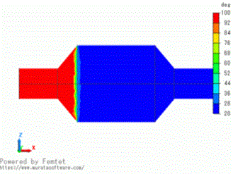 |
5 [s] 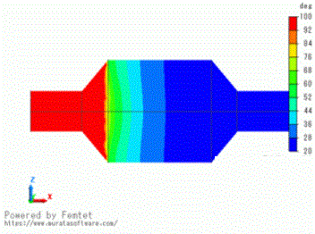 |
20 [s] 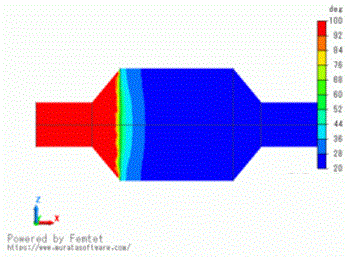 |