|
Home / Examples / Piezoelectric Analysis [Rayleigh] / Example 27: Transient Analysis of Pressure Drive
Example 27: Transient Analysis of Pressure Drive
General
-
Transient analysis is explained in this example.
-
Obtain this session's project file. (Right-click and choose 'Save link as')
Model 1, "ImplicitMethod", is a transient analysis model. Simulation Time: 1 min 15 sec.
Model 2, "ResonantMethod", is a transient analysis model with the resonant analysis.
Model 3, "ResonantMethod_auto", is a transient analysis model with the resonant analysis, the automatic timestep setting being applied.
The difference between models 1 and 2 is only the analysis conditions.
-
Results will vary depending on Femtet version and the PC environment.
-
Unless specified in the list below, the default conditions will be applied.
-
Transient analysis is available in an optional package. However, transient analysis using resonant mode is not optional.
Analysis Space
|
Item |
Settings |
|
Analysis Space |
2D |
|
Model Unit |
mm |
Analysis Conditions
|
Item |
Settings |
|
Solver |
Piezoelectric Analysis [Rayleigh] |
|
Analysis Type |
Transient Analysis |
|
Transient Analysis Using Resonant Mode (Model 1) |
Deselected |
|
Transient Analysis Using Resonant Mode (Models 2 and 3) |
Selected |
The settings on the transient analysis tab are required.
For model 2, the settings on the resonant analysis tab are required.
The resonant analysis tab is set up as follows.
|
Tab |
Setting Item |
Settings |
|
Resonant Analysis (only for models 2 and 3) |
Number of Modes |
3 |
|
Approximated Frequency |
0 [Hz] |
|
|
Transient Analysis > Manual (Model 1 and Model 2) |
Timestep |
Select [Manual] |
|
Output Interval |
1 |
|
|
Number of Calculation Steps |
100 |
|
|
Transient Analysis > Automatic (Model 3) |
Timestep |
Select [Automatic] |
|
Mesh |
Meshing Setup/Element Type |
Select [Rectangle] (**) |
The standard timestep is set as [period/10], but to be on the safe side, it is set as [period/25] to give more steps.
For model 3, the timestep is automatically determined from the results of resonant frequencies.
One-tenth of the period corresponding to the highest resonant frequency is used as the timestep. (The number of divisions per cycle can be changed)
(**)The triangle is the standard element for the 2D analysis. In this example, rectangle is selected to demonstrate that the rectangular mesh also can be used.
Model
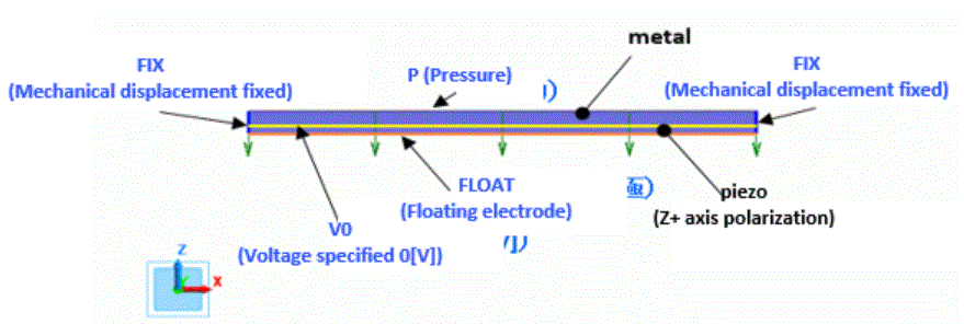
Body Attributes and Materials
|
Body Number/Type |
Body Attribute Name |
Material Name |
|
0/Face |
METAL |
001_Al * |
|
1/Face |
PIEZO |
000_P-4 * |
* Available from the material DB
Boundary Condition
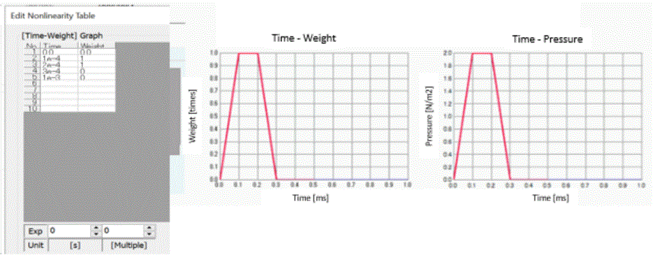
The time dependency of the applied pressure is defined by weight function.
|
Boundary Condition Name/Topology |
Tab |
Boundary Condition Type |
Settings |
|
P/Edge
|
Mechanical |
Pressure |
2 [Pa] Select [Time Dependency] Enter [Weight Function] as shown in the diagram below.
|
|
Electric |
Electric Wall |
Magnetic Wall |
|
|
V0/Edge |
Mechanical |
Free |
|
|
Electric |
Electric Wall |
Specify electric potential: Electric Potential 0 [V] |
|
|
FLOAT/Edge |
Mechanical |
Free |
|
|
Electric |
Electric Wall |
Floating Electrode |
|
|
FIX/Edge |
Mechanical |
Displacement |
UX=0.0, UY=0, UZ=0 |
|
Electric |
Magnetic Wall |
|
Below are the [Weight Function] table of the pressure-specified boundary condition and graphs. Since the input pressure is 2 [Pa] and the maximum weight is 1, the maximum value of the applied pressure is also 2 [Pa].
Results (Model 2: Resonant Analysis)
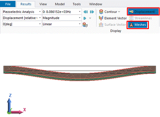
The displacement diagram is shown below with the mesh diagram.
Results (Model 2: Transient Analysis)
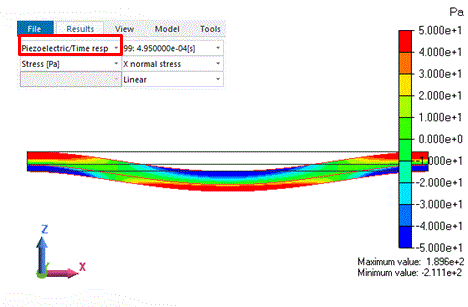
Shown below is the X normal stress of the result of the last analysis time.
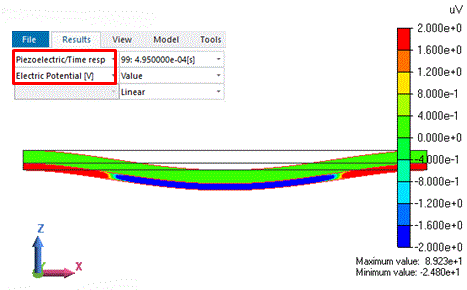
Shown below is the electric potential distribution of the result of the last analysis time.
Results (Comparison of Models 1 and 2)
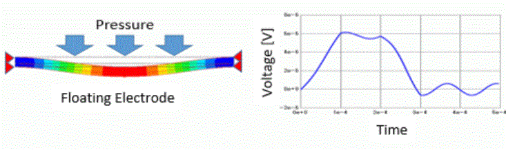
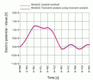
The electric potential change of the floating electrode over time is shown in the graph below.
The horizontal axis is the modes. The coordinates on the floating electrode are specified. The coordinates can be obtained with the mouse.
The overlapping plots of results of models 1 and 2 are shown below. They match very well.
- See here for creating graph.
-
For the [Type] on the [Field Graph Setting] tab , select [Horizontal Axis: Mode (frequency, time, step, etc)]
-
For overlapping plots, see [drag-and-drop on the graph window].
-
The electric potential of the floating electrode can be plotted from the data in the result table.
Results (Comparison of Models 2 and 3)
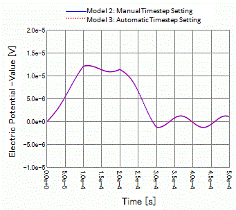
Models 2 and 3 are also compared.
The models with the timestep specified manually and automatically match very well.