Home / Technical Notes / Magnetic analysis / Differential Equations in Harmonic Magnetic Analysis

Differential Equations Solved in the Magnetic-Harmonic Analysis

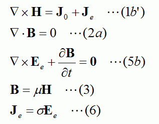
H: Magnetic field

B: Magnetic flux density

J0: Forced current density

Je: Induced current density

Ee: Induced electric field

μ: permeability

σ: Conductivity

 

Equations (1b), (2a) and (3) are solved for the given J and boundary conditions, and H, B, Ee and Je are obtained.

 

 

It is selectable in the analysis condition whether or not Je is generated in the area where J0 exists.

If Je is generated, the resulting current density is J0 + Je. In that case, the skin effect and the proximity effect are taken into account.

 

 

 

Equation (1b') is Ampere's law. * Note 1

Equation (2a) is Gauss's law for magnetism.

Equation (5b) is Faraday's law of induction. * Note 2

 

Equation (3) defines the relation between the material's magnetic flux density and field.

Equation (6) defines the relation between material's current density and electric field.

 

 

 

Note *1

 

The extended form of Equation (1b') is Maxwell-Ampere equation given by (1a'):

 

μ: permeability

B: Magnetic flux density

D: Electric flux density

J0: Forced current density

Je: Induced current density

 

In harmonic analysis, we should be using Equation (1a').

Instead, we are using Equation (1b') assuming the frequency is low and the time derivative of D is nearly 0. For high-frequency simulations where dD/dt cannot be ignored, use solver Electromagnetic Analysis (Hertz).

 

 

Note *2

 

Equation (5b) is Faraday's law with induction. When J0 exists, the electric field which generates J0 must exist in the analysis space. Equation (5b) is, therefore, extended to Equation (5a):

 

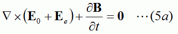
E0: Electric field generating forced current

Ee: Induced electric field

B: Magnetic flux density

 

In Femtet, Equation (5b) is used instead of (5a), so ∇xE0 = 0. That means E0 is equal to the gradient of electric scalar potential φ0 in this case.

 

 

 

Governing Equation

 

Solver "Gauss" solves equations which are derived from Equations (1b'), (2a), (5b), (3), and (6).

 

By introducing electromagnetic potentials (A, φe), B and Ee are given by Equations (2b) and (5c):

 

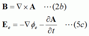
B: Magnetic flux density

A: Magnetic vector potential

Ee: Induced electric field

φe: Electric scalar potential

 

These equations satisfy Equation (2a) and (5b) automatically.

 

Equations (1b'), (3) and (6) are combined, and Equation (7) is obtained.

 

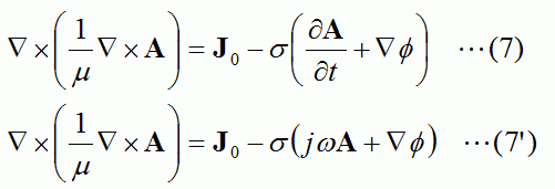
μ: permeability

A: Magnetic vector potential

J0: Forced current density

σ: Conductivity

φe: Electric scalar potential

j: Imaginary unit

ω: Angular frequency

 

 

 

For a given angular frequency ω, Equation (7) becomes Equation (7').

Femtet Solver "Gauss" solves Equation (7') and obtains electromagnetic potentials (A, φe).

Then B, Ee and Je are calculated from Equations (2b), (5c) and (6).

 

 

You don't need to define J0 for the full analysis space. From the given conditions, Femtet deduces J0's space distribution

and gives that in Equation (7').

 

 

Some boundary conditions must be given to solve Equation (7'). For example,

 

Magnetic wall: The magnetic flux density B (∇×A) meets the magnetic wall ar right angle. The magnetic flux density B and the normal vector n of magnetic wall run in the same or opposite direction.

Electric wall: The magnetic flux density B (∇×A) and the electric wall run in parallel. The magnetic flux density B meets the normal vector n of electric wall at right angle (B・n=0).