|
Home / Examples / Piezoelectric Analysis [Rayleigh] / Example 17: Deformed Meshes
Example 17: Deformed Meshes
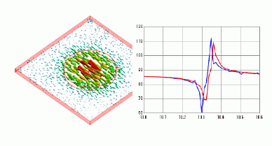
General
-
The impedance change due to thermal load is solved with deformed meshes. See Analysis with Deformed Meshes for the details of analysis operation using deformed meshes.
-
This example is based on the example 9: Thickness Shear Mode.
-
Copy the analysis model “ray_ex9” into the project and name it "Static". Change the analysis condition to Thermal load and obtain the deformed shape.
-
Copy the analysis model “ray_ex9” into the project and name it "Deformed mesh". This analysis model is solved with the obtained deformed meshes. Analyze the impedance.
-
Obtain this session's project file. (Right-click and choose 'Save link as') Simulation Time: 2 min 20 sec.
-
Results will vary depending on Femtet version and the PC environment.
Preparation
Open Project "ray_ex09.femprj > Project tree pane > right click on "ray_ex09" > Copy into Project > name it "Static". Go to Project tree pane again > right click on "ray_ex09" > Copy into Project > name it "Deformed mesh". There will be 3 analysis models in total.
Analysis Conditions of "Static"
|
Item |
Settings |
|
Solver |
Piezoelectric Analysis [Rayleigh] |
|
Analysis Type |
Static Analysis |
|
Options |
Thermal Load |
|
Output Setting |
Select [Impedance] |
|
Tab |
Setting Item |
Settings |
|
Thermal Load Tab |
Reached Temperature |
100 [deg] |
|
Reference Temperature (Non-Stress Temperature) |
20[deg] |
Analysis Conditions of "Deformed mesh"
|
Item |
Setting |
|
Solver |
Piezoelectric Analysis [Rayleigh] |
|
Analysis Type |
Harmonic Analysis |
|
Options |
N/A |
|
Tab |
Setting Item |
Setting |
|
Harmonic Analysis |
Sweep Values |
Minimum: 18.0×10⁶ [Hz] Maximum: 18.6x10⁶ [Hz] |
|
Sweep Type |
Select [Linear Step by Division Number]. Division: 50 |
|
|
Result Import |
Import Type |
Deformed Shape |
|
Specify Results |
Select [Specify analysis model] Select [Static analysis] |
Graphical Objects
The same as the example 9: Thickness Shear Mode
Body Attributes and Materials
The same as the example 9: Thickness Shear Mode except that Coefficient of Linear Thermal Expansion is used to take the thermal load into account for the static analysis.
Boundary Condition
The same as the example 9: Thickness Shear Mode
Procedure
1. Analysis model "ray_ex9" > Run Mesher/Solver > Save Project. (This is for later comparison)
2. Analysis model "Static" > Run Mesher/Solver > Save Project (This is for obtaining mesh shapes thermally expanded)
3. Analysis model "Deformed mesh" > Run Solver (Harmonic analysis is performed with the meshes obtained in 2)
Press [Run Solver with Existing Meshes], and select “static analysis(deformed meshes).pdt” in the result folder. This is a result file of 2.
-
In 2, if a result file of the deformed mesh is not output, select [Save the deformed mesh results when saving the calculation result] in GUI Setting, and execute 2.
Results
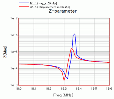
How the frequency response of impedance shifts due to the thermal load is examined below.
(1) Show the frequency response of impedance of the analysis model “ray_ex9”.
(2) Show the frequency response of impedance of the analysis model “Deformed meshes”.
(3) Since the graph data can be moved on the Graph tree, move the graph data of (2) onto the graph icon of (1) (“GC01”) to plot on the same graph.
The shift of resonant frequency due to the thermal expansion is observed.
- The frequency response of impedance can be plotted from an S(Y) parameters graph.
- For overlapping plots, see [Drag-and-Drop on the Graph Window].