Home / Examples / Acoustic Analysis [Mach] / Example 3: Interference of Sound Waves (2D)

Example 3: Interference of Sound Waves (2D)

General

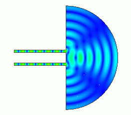
• The interference of sound waves from two sources is analyzed.
   

• The interference pattern is solved.
  

• [Field Superposition Setting] function is used to observe the change in the field when the phase of the driving source is changed.
   

• Unless specified in the list below, the default conditions will be applied.
   

• Obtain this session's project file. (Right-click and choose 'Save link as')




• Results will vary depending on Femtet version and the PC environment.

 

Analysis Space

Item	Settings
Analysis Space	2D
Model Unit	m

 

Analysis Conditions

Item	Settings
Solver	Acoustic Analysis [Mach]
Analysis Type	Harmonic Analysis
Options	N/A

 

The harmonic analysis tab is set up as follows.

The sound waves propagate outside the analysis region. Therefore, the [open boundary] condition below is applied initially.

The default conditions will be applied.

Tab	Setting Item	Settings
Harmonic analysis	Frequency: Sweep Values	Minimum: 1 [kHz] Maximum: 2 [kHz] Number of Divisions 1
	Frequency: Sweep Type	Linear Step by Number of Divisions
	Frequency Sweep	Discrete Sweep
	Enable Each Port's Individual Weight Setting for the Superposed Field Display	Select
Open Boundary Tab	Type	Absorbing Boundary
	Order of Absorbing Boundary	1st-order
	Coordinates of Origin	x = z = 0

 

Model

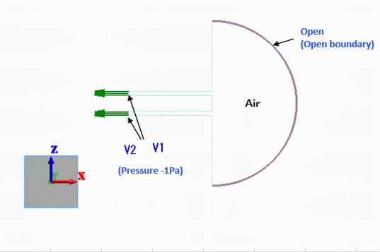
The model is created in 2D. A semi-circle and two rectangular sheet bodies form the air. The pressure boundary condition is set to the sound generating portion.
The open boundary condition is set to the perimeter of the semi-circle.

Body Attributes and Materials

Body Number/Type	Body Attribute Name	Material Name
5/Sheet	Air	000_Air(*)

* Available from the material DB

Boundary Conditions

The boundary conditions of open boundary and pressure are set.

 

Boundary Condition Name/Topology	Tab	Boundary Condition Type	Settings
Open/Face	Acoustic	Open Boundary
V1/Face	Acoustic	Pressure	-1 [Pa]
V2/Face	Acoustic	Pressure	-1 [Pa]

 

Results

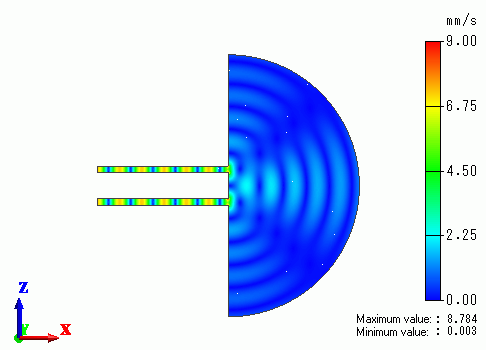
Shown below are the gradation contours of the particle speed at 1000 [Hz] and 2000 [Hz].

 

Frequency: 1000 [Hz]

 

Frequency: 2000 [Hz]

 

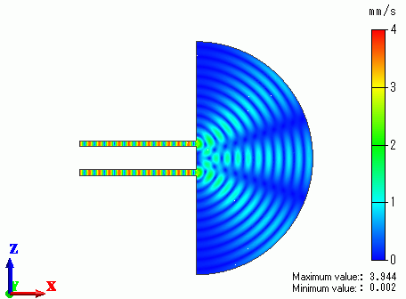
The interference pattern varies with the frequency.

 

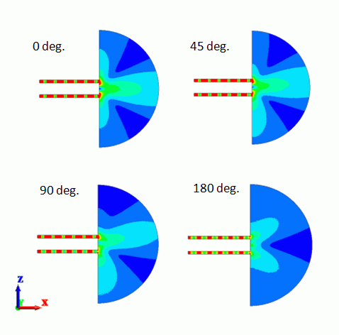
Next, let's change the coefficient in the Field Superposition Setting and see its effect. Open the [Field Superposition Setting] dialog box.

The boundary condition names for each driving source (V1, V2) and the corresponding coefficients will appear in the (MAG PHASE) formats.

Initially, (MAG=1.0, PHASE=0.0[deg]) will show up. In this example, we change PHSE of V2 to 0,45,90,180 [deg]

and see the change in the field.

The figures below are with the fields set to 1000 [Hz], Particle velocity, Magnitude, Absolute, and Linear.

The minimum value of the contour diagram is set to 0 [mm/s] and the maximum value to 5 [mm/s].

For easy viewing, the contour is set with [Gradation contour with color division] selected.

By changing the PHASE, the pattern of the contour is changed. The directivity changes according to the pattern change of the contour as shown below.

 

 

 

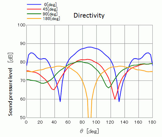
The calculation conditions of the directivity are as follows.

Observation point: r=1 [m], φmin=0.0 [deg], φmax=0.0 [deg], φstep=0, θmin=0.0 [deg], θmax=180 [deg], θstep=60

Select Sound Pressure Level [dB] for Display and select YZ plane for Plane of Symmetry. (Calculation is based on the assumption that the wall parallel with Z axis is extending a long distance)

Select Theta for Horizontal Axis.