Home / Examples / Electromagnetic Analysis [Hertz] / Example 7: Dipole Antenna

Example 7: Dipole Antenna

General

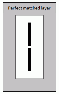
The perfectly matched layer (PML) is used to analyze a dipole antenna.
Unless specified in the list below, the default conditions will be applied.
Obtain this session's project file. (Right-click and choose 'Save link as')
Results will vary depending on Femtet version and the PC environment.

[How to Reduce the Calculation Time]
The animation for the radiation characteristics is created at the end of this session.

Analysis Space

Item	Settings
Analysis Space	3D
Model Unit	mm

Analysis Conditions

Item	Settings
Solver	Electromagnetic Analysis [Hertz]
Analysis Type	Harmonic Analysis

Harmonic Analysis tab and Open Boundary tab are set as follows.

Tab	Setting Item	Settings
Mesh Tab	Element Type	1st-order Element
	Adaptive Meshing	Select [Apply adaptive meshing].
	Frequency-Dependent Meshing	Reference Frequency: 5x109 [Hz] Select [The conductor bodies thicker than the skin depth constitute the boundary condition]. ANTENNA is thicker than the skin depth. Its surface will be set with the proper boundary condition based on the material automatically.
Harmonic analysis	Sweep Type	Select [Linear Step by Number of Divisions]
	Sweep Setting	Minimum: 3×109 [Hz] Maximum: 6x109 [Hz] Number of Divisions: 100
	Sweep Setting	Select Fast Sweep S-parameter tolerance: 1x10-3
	Input	1.0 [W]
Open boundary	Type	PML (Perfectly Matched Layers)
Open boundary	Thickness of PML Layer	0.2 Wavelength *

* It is 0.3 by default. To shorten the calculation time, it is changed to 0.2.

Model

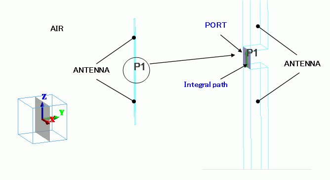
Two conductor rods are placed in the air box. The rods are rectangular solid bodies.

Set the port boundary condition on a sheet body connecting the conductor rods.

Body Attributes and Materials

Body Number/Type	Body Attribute Name	Material Name
3/Solid	ANTENNA	104_Stainless_steel *
4/Solid	ANTENNA	104_Stainless_steel *
5/Sheet	Imprinting body
6/Solid	AIR	000_Air(*)

* Available from the material DB

Boundary Conditions

Boundary Condition Name/Topology	Tab	Boundary Condition Type	Settings
PORT/Face	Electric	Port	Reference Impedance: Select [Specify] and enter 50 [Ohm]. Number of Modes Number of Precalculated Modes: 5 Number of Modes Used in the Actual 3D Analysis: 1 Select modes: None
OPEN/Face	Electric	Open Boundary	Select PML on the open boundary tab of the analysis condition setting.
Outer Boundary Condition	Electric	Electric Wall

Results

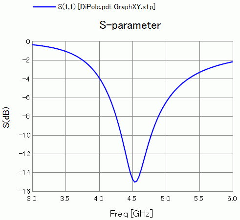
S-parameter S11 at the feeding point is shown below.

It is matched at about 4.5 GHz.

How to Display Graph
On the [Results] tab, go to and click ▼ at the right side of [Show Characteristics Chart]. Click [S/Y Parameters] on the submenu.

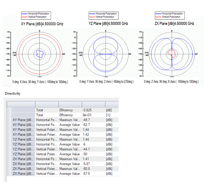
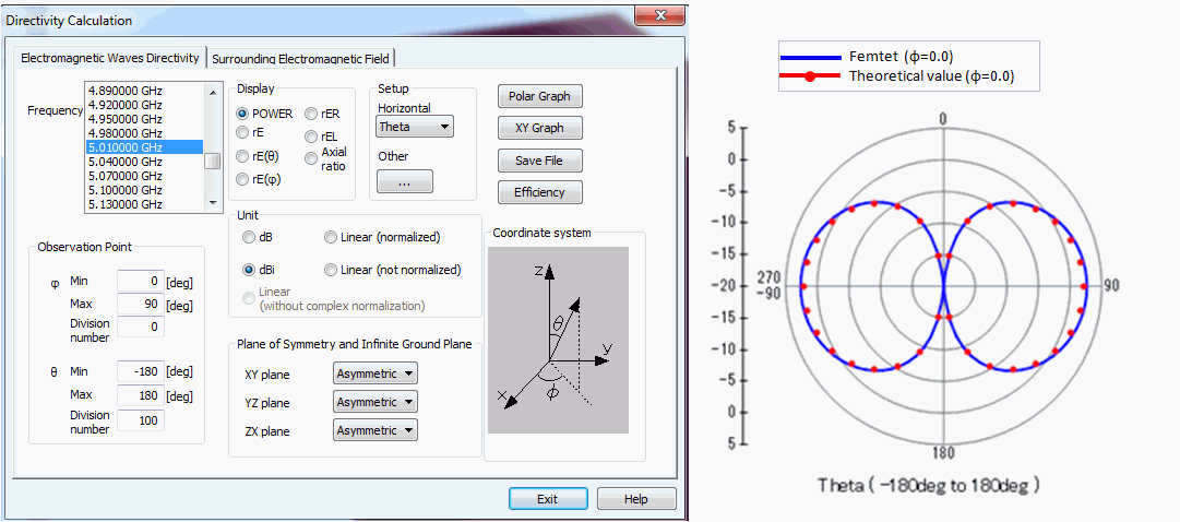
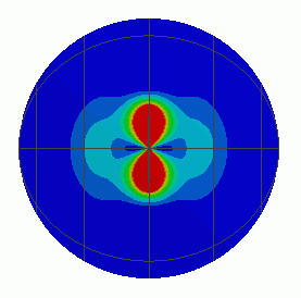
The radiation patterns and efficiency of the antenna at 4.5 GHz are shown below.

How to Display
On the [Results] tab, go to and click ▼ at the side of [Show Characteristics Chart]. Click [Directivity Graph] on the submenu.
See [[Simple Mode] Electromagnetic Waves Directivity] for more information.

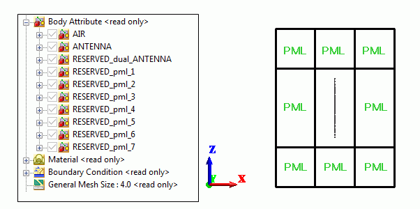
The perfectly matched layers with body attributes of RESERVED_PML_xx are generated automatically.

The green characters of "PML" below will not be displayed on the results window. They are just for helping your understanding.

Comparison with the Theoretical Results

The theoretical results and radiation pattern of the half wavelength dipole antenna are compared. The calculation condition is as follows.

- Frequency 5.01 GHz (Select the frequency so as to make the length of antenna 1/2 wavelength)

- Radiation pattern measured on the XZ plane. Settings of the observation point are; φ(minimum value: 0 [deg], maximum value: 90 [deg], number of divisions: 0), θ(minimum value: -180 [deg], maximum value: 180 [deg], number of divisions: 100).

- Display: POWER, unit: dBi

- [Received power referenced] for the [Gain Type] is selected on the [[Detailed Mode] Electromagnetic Waves Directivity] tab. Operation is as follows. If you press the [Other] of the Directivity dialog box, [Directivity Setting] dialog box will appear. Then, [received power referenced] is selected for the gain type.

How to Create the Animation

Animations tend to look better when the larger ambient zone is set, e.g..more than one wavelength.
However, that might increase the number of meshes.
To suppress the number of meshes, try the absorbing boundary instead of PML.

The animation will look better with smaller meshes.

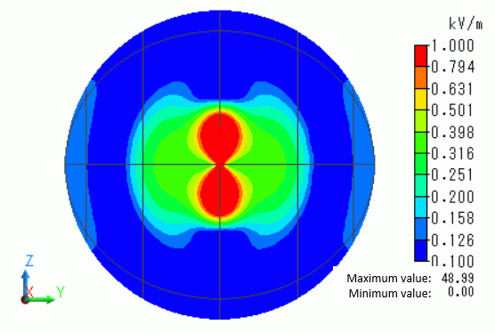
The left figure is the model. The right figure is the contour of the electric field sectioned by the plane encompassing the antenna.

# Setting Item

Analysis Condition Setting -> Open Boundary tab -> Absorbing Boundary

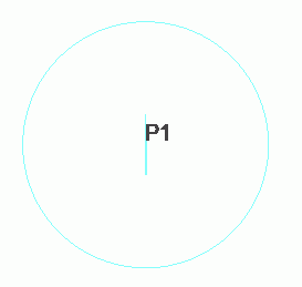
Modeling -> Air Sphere -> Radius: 60

Modeling -> Mesh Size: 4

Analysis Condition Setting -> Mesh tab -> Meshing Setup -> 2nd-order Element

# Results Window

[Solver]: Electromagnetic Analysis
[Mode]: 4.5 GHz
[Field Type]: Electric Field
[Component]: Magnitude
[Phase]: 90 deg *
[Scale]: Log

* This setting is for the better look of contour. It does not affect the animation.

# Contour tab in Graphics Setup

Deselect [Automatic]
Minimum value: 100
Maximum value: 1000

# Cross Section

The contour of cross section that is in the center of the ambient air and parallel to the YZ plane is shown in the right diagram above.
The animation displays the electromagnetic waves radiation.

See [How to Create Animation] for detail.

Obtain this file. (Right-click and choose 'Save link as')
Results will vary depending on Femtet version and the PC environment.

Make the mesh size bigger: See [Mesh tab] for details.
Select 1st-order element: See [Mesh tab] for details.
Disable adaptive mesh: See [Mesh tab] for details.