High-Level Setting Tab

Setting Item

Notes

Nonlinear Analysis

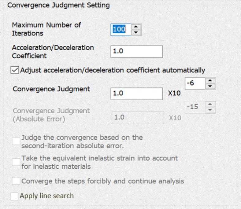
Convergence Judgment Setting
(Except for stress and fluid analysis)

Iterative calculations are repeated until the convergence is achieved in nonlinear analysis.
It is judged that the convergence is achieved
when the tolerance of calculation becomes less than the value in [Convergence judgment].

The calculation will stop when the iterations reach the [Maximum number of iterations].

If the nonlinear slope is too steep, the iterative calculations might not converge.
In such a case, adjust the [Acceleration/deceleration] factor. This function is available for the electrostatic analysis, the plating analysis,
the magnetic analysis, and the thermal analysis.
If it is 0.1, for example, the iteration step will be one tenth of the usual step.
The possibility of convergence increases but the number of iterations also increases.
In this case, the number of iterations will be 1/0.1 = 10 times more.

Select "Adjust acceleration/deceleration factor automatically"
to let Femtet adjust the factor automatically.

[Maximum number of iterations] is an integer greater than 0.
The significand of [Convergence judgment] is a real number greater than 0.
[Acceleration/deceleration] factor is a real number greater than 0.
Not available for the resonant analysis.

[Apply line search] is available only for the magnetic transient analysis.

The line search determines the relaxation factor used in the Newton-Raphson method so that the residual of the matrix equation is close to the minimum.

This function is to accelerate the convergence in the nonlinear magnetic analysis.

In some cases, the calculation speed may be several times faster, but not always. So the default setting is OFF.

Try Newton-Raphson method if the convergence is poor.

If the calculation doesn't converge in nonlinear analysis, try the following:
1. Increase the maximum number of iterations.
2. Increase the convergence judgment value (tolerance).
3. Reduce the deceleration factor (only in the electrostatic analysis, plating analysis, magnetic analysis, thermal analysis, and electric-thermal coupled analysis).

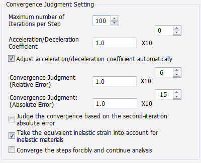
Nonlinear Analysis

Convergence Judgment Setting
for Stress Analyses

To realize the nonlinearity, the displacement or the load is divided into some small steps and
increased gradually.
Iterative calculations are done for each step.
See [The Newton-Raphson Method and Convergence Judgment in Stress Analysis].

The convergence is judged by [absolute error] (= the sum of squared displacement of all nodes) and
[relative error] (= the absolute error of the current iteration divided by that of the first iteration)

The calculation is considered to have converged when either the relative error or
the absolute error becomes smaller than the value for convergence judgment.

The significand of [Convergence Judgment (Relative Error)] is a real number greater than 0.
The significand of [Convergence Judgment (Absolute Error)] is a real number greater than 0.

If "Judge the convergence based on the second-iteration absolute error" is selected,
the convergence will be judged by the second-iteration absolute error instead of the first-iteration absolute norm.

If "Take the equivalent inelastic strain into account for inelastic materials" is selected,
the convergent will be judged by the absolute or relative error of the equivalent inelastic strain
as well as that of the displacement.
It will be considered to be converged only when both the displacement and the equivalent inelastic strain are converged.

The calculation will stop as soon as the iterations reach the entered maximum number.

[Maximum number of iterations per step] is an integer greater than 0.

If the calculation doesn't converge,
reducing [Acceleration/deceleration] factor might help.
If it is 0.1, for example, the iteration step will be one tenth of the usual step.
The possibility of convergence increases but the number of iterations also increases.
In this case, the number of iterations will be 1/0.1 = 10 times more.
In some cases, increasing the factor might help the convergence.
Select "Adjust acceleration/deceleration factor automatically"
to let Femtet adjust the factor automatically.

[Acceleration/deceleration] factor is a real number greater than 0.

If [Converge the steps forcibly and continue analysis] is selected,

the result closest to convergence in the iterations before calculation stopped will be used as an optimum solution to continue analysis.

Although the calculation accuracy will be lower, this is useful in the cases the calculation doesn't converge or takes long time to converge

See [Example 56: Buckling Analysis of Bimetal Switch]

Nonlinear analysis

Convergence Judgment Setting
(For fluid analysis)

Iterative calculations are repeated until the convergence is achieved in the fluid and fluid-thermal analysis.
It is judged that the convergence is achieved
when the tolerance of calculation becomes less than the value in [Convergence judgment].

Different values for convergence judgment can be set for fluid analysis and thermal analysis.

The calculation will stop when the iterations reach the [Maximum number of iterations].

If iterative calculation does not converge in the thermal analysis, use [Acceleration/Deceleration factor].
If it is 0.1, for example, the iteration step will be one tenth of the usual step.
The possibility of convergence increases but the number of iterations also increases.
In this case, the number of iterations will be 1/0.1 = 10 times more.

Select "Adjust acceleration/deceleration factor automatically"
to let Femtet adjust the factor automatically.

[Maximum number of iterations] is an integer greater than 0.
The significand of [Convergence judgment(heat)] is a real number greater than 0.

The significand of [Convergence judgment(fluid)] is a real number greater than 0.

[Acceleration/deceleration] factor is a real number greater than 0.

If the calculation doesn't converge in fluid analysis, try the following:
1. Increase the maximum number of iterations.
2. Increase the convergence judgment value (tolerance).
3. Reduce the relaxation factor at [Detailed Setting of Fluid Analysis] on the [Fluid analysis tab].

If the calculation doesn't converge in thermal analysis, try the following:
1. Increase the maximum number of iterations.
2. Increase the convergence judgment value (tolerance).
3. Reduce the deceleration factor.

Nonlinear Analysis

If non-convergence, set a finer timestep.

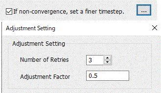
[If non-convergence, set a finer timestep]

If the calculation didn't converge with this function enabled, the load increment is adjusted automatically and the calculation is redone

It is preselected by default.

Assume that the number of the substeps is 20 and the adjustment factor is 0.5. The load increment will be 5% (1/20) initially. If the calculation of a substep doesn't converge, it will be redone with the load increment multiplied by 0.5 into 2.5% (5% x 0.5).

If it doesn't converge yet, another recalculation will be done with the load increment multiplied by 0.5 into 1.25% 2.5% x 0.5). These recalculations will be repeated until they converge or the number of calculations reaches [Number of Retries].

[Number of Retries] is a positive integer. (0 not inclusive)
[Adjustment factor] is a real number greater than 0.

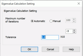
Eigenvalue Calculation

Specify the maximum number of iterations for the eigenvalue calculation and the convergence tolerance.

If the [Maximum number of iterations] is automatic, the iterations are set automatically.
[Maximum number of iterations] is an integer greater than 0.
The significand of [Tolerance] is a real number greater than 0.
Available for the resonant or buckling analysis only.

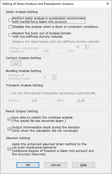
Stress Analysis/Piezoelectric Analysis Setting

[Static Analysis Setting]

If [Perform static analysis in acceleration environment with inertial force taken into account] is selected,
acceleration/angular acceleration are given to the body to counterbalance the force/torque which are not balanced in the body.
Calculation is performed on the external force and moment of inertia in the balanced state. (Inertia relief function)

The density is required to be set on the [Density tab].

This is available for the static stress analysis and the piezoelectrostatic analysis.

For detail, see technical note [Balance of Forces and Torques in the Static Analysis].

If [Stabilize the analysis which is short of constraint conditions] is selected, the analysis is stabilized even when there are bodies short of constraint conditions.

This is effective for the contact analysis in which bodies are not fully constrained.

If [Replace the body out of analysis domain with low-stiffness dummy material] is selected,
the bodies that are out of the analysis domain can be treated differently in the static single-step analysis and the thermal load analysis.
It is deselected by default.

If [Replace the dead body with low-stiffness dummy material] is selected,
death setting of the bodies can be changed in the multi-step analysis and multi-step thermal load analysis in the static stress analysis.
It is preselected by default.

Refer to [Stress-Static Analysis] of the Technical Notes for the details of birth/death.

[Stiffness adjustment factor] can be changed if [Replace the body out of analysis domain with low-stiffness dummy material] or [Replace the dead body with low-stiffness dummy material] is selected.

Young's modulus of the bodies out of analysis domain or dead bodies is multiplied by this value.
The default value is 1.0 x 10^-6, which is significantly small.

[Contact Analysis Setting]

Click this button. The [Contact Analysis Setting] dialog box will appear.

[Buckling Analysis Setting]

[Number of buckling modes] is set. The number is a positive real number. (0 not inclusive)

Transient Analysis Setting

If [Set the time-domain integration parameters automatically] is selected, the integration parameters of Newmark method are set automatically. If deselected, the parameters (Gamma and Beta) can be set manually.

[Result Output Setting]

Some nonlinear analyses (elasto-plastic, creep, viscoelasticity, and contact) require intermediate data for restart analysis.

If [Save Data to Restart Nonlinear Analysis] is selected, nonlinear analysis which requires intermediate data can be restarted.
The results file size becomes larger because it stores the intermediate data.
If the option is deselected, the results file size becomes smaller although the restart analysis cannot be performed.

[Output intermediate result during the iteration]

When selected, the intermediate result is output if the calculation did not converge. The result file size becomes larger.

If deselected, the intermediate result is not output. The last non-convergent result or diverged result is only output.

[Apply Enhanced assumed strain method to 1st-order hexahedral (rectangular) elements]

If selected, Enhanced assumed strain method is applied to increase the simulation accuracy for 1st-order 3D hexahedral or 2D rectangular elements. (Not supported for piezoelectric analysis)

If deselected, formulation of enhanced strain is disabled and the calculation speed will be faster but the simulation accuracy may be much poorer.

See Enhanced Assumed Strain Method of technical note for more information.

Surface-to-Surface Radiation Setting

In the thermal analysis, if [Surface-to-surface (accuracy prioritized)] is selected for the radiation setting,
the radiation surface check and the view factor calculation can be specified.

A solver to calculate the radiation is specified in [Radiation Solver].

If [Face - Face (Time Prioritized)] is selected, the calculations will be faster, but the accuracy will be deteriorated.

If [Point - Face (Accuracy Prioritized)] is selected, the accuracy will be higher, but the calculations will take longer time.

The default setting is [Face - Face (Time Prioritized)].

A solver to calculate the radiation is specified in [Radiation Solver].

If [Face - Face (Time Prioritized)] is selected, the calculations will be faster, but the accuracy will be deteriorated.

If [Point - Face (Accuracy Prioritized)] is selected, the accuracy will be higher, but the calculations will take longer time.

The default setting is [Face - Face (Time Prioritized)].

[Radiation Surface Check Method] allows you to directly specify the method for checking radiation surfaces.
* if [Automatic] is selected: For 3D analysis, Mapping method or Hemicube method is applied.
For axisymmetric analysis, Triple-loop method is applied.
For 2D analysis, Triple-loop method is always applied.

Only if [Face-Face (Time Prioritized)] is selected, the Hemibube method can be selected.

The accuracy of the mapping method can be adjusted in [Mapping Method Setup].
Higher mapping resolution provides higher accuracy. However, the calculation takes longer time. The tolerance of distance check affects the accuracy of the calculation, while it does not affect the calculation time. The most appropriate tolerance providing the high accuracy depends on the mapping resolution and the features of the model (mainly the mesh size).
In most cases, the mapping method provides almost the same accuracy as the triple-loop method with enough mapping resolution and appropriate tolerance.

In [Hemicube Method Setup], the Hemicube resolution can be adjusted.

You can specify it only if the Hemicube method is selected in [Radiation Surface Check Method].

The resolution is the number of pixels per edge of a face of the hemicube (64 by default).

Higher resolution will improve rendering accuracy to increase calculation accuracy.

High-performance discrete GPUs can shorten calculation time.

If [Evaluate the difference between triple-loop and mapping methods] is selected, the both methods are performed in the radiation surface check, and the difference (unit: %) between them is obtained.

This setting is available only when the radiation solver is set with [Point - Face (Accuracy Prioritized].

The thermal analysis following the radiation surface check uses the results of the triple-loop method.
If the difference is large, the results of the mapping method might be larger compared to that of the triple-loop method.

See Technical Note [Radiation Surface Check].

In [Calculation Method of View Factor], the method to calculate the view factor of the radiation surfaces.

If the solver is set with [Face-Face (Time Prioritized)] and the mapping or Hemicube method is used, this setting is not required because the view factor is calculated by the mapping method or Hemicube method without element surface integration.

Surface integral is required to calculate the view factor.

There are analytical integration and numerical integration for the surface integral. Analytical integration provides high accuracy. Numerical integration provides fast calculation.

Depending on the state of the radiation surfaces, either analytical integration or numerical integration is automatically selected in [Automatic (analytical integration and numerical integration jointly used)] .
High accuracy in fast calculation will be obtained.
[Accuracy Prioritized (analytical integration)] provides the high accuracy, but takes long time.
[Time Prioritized (numerical integration)] provides fast calculation, but the accuracy is degraded.
Especially, if the radiation surfaces are close in relation to the mesh size, or if the mesh size is large in relation to the distance between the radiation surfaces, the accuracy will notably be degraded.

The default setting is [Automatic (analytical integration and numerical integration jointly used)] .

Thermal Analysis Setting

Set the correction factor for convection.

The factor adjusting heat dissipation by natural or forced convection is set in this dialog box. It is also used for non-air fluids such as water and solvents. The factor is 1.0 for the heat dissipation into air at 25 °C.

・Automatic Calculation

Select a fluid for heat dissipation. The correction factor of convection is automatically calculated based on the Femtet material database information of the selected fluid material.

For the coupled analysis with the simple fluid analysis, the menu of fluid selection will not appear. Instead, the fluid material selected in the material property setting is set to the fluid for heat dissipation.

If [Temperature Dependency Taken into Account] is selected, the temperature dependency will be taken into account for the calculation of correction factor for convection. Refer here for the equations.

The material properties of the selected fluid material can be edited for more detailed material properties.

For instance, the temperature dependency data of density is not registered in the material database in Femtet. If the temperature dependency data of density is input in the material property setting, the correction factor for convection can be calculated more accurately.

See [How to Set Body Attribute/Material Property] or [Density Tab] for the editing.

・Manual Setting

The correction factor is used to match the simulation result and the measurement result.

The correction factor can be fixed by performing a simulation and making a measurement for a reference model and comparing the results. Refer here for the setting.

This setting is applicable for thermal analyses [Watt] or Watt-coupled analyses under the natural-convection (automatic calculation) boundary condition

also for simple fluid-thermal analyses [Pascal-Watt]

Result Output Setting

When selected, the intermediate result is output if the calculation did not converge. The result file size becomes larger.

If deselected, the intermediate result is not output. The last nonconverged result or diverged result is only output.

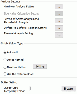
Matrix Solver

Matrix Solver Type

• For the magnetic transient analysis, only iterative method is used.

The iterative method of the algebraic multi grid is performed in the analyses below for fast calculation.

・ Thermal Analysis

・ Simple Fluid Analysis

The iterative method of the domain decomposition is performed in the analyses below for fast calculation.

・ Stress Analysis (Static Analysis)

Note that the domain decomposition method is not applicable under the conditions below in the stress static analysis.

・ Contact surface, simple contact, joint load, spring connection, rigid face, or bond boundary condition is applied.

・ Shell elements are applied.

The algebraic multi grid method requires an optional license.

The domain decomposition method requires an optional license.

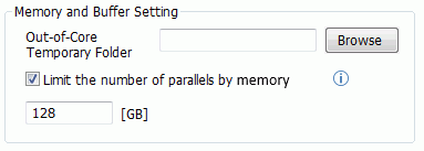
Buffer Setting/Memory and Buffer Setting

The direct method takes the large memory space during the calculation. Therefore a certain portion of the main memory of the PC is allocated to perform the direct method. "Buffer size" is this allocation size.
If the buffer size is not large enough for the calculation, the hard disk will be used additionally.

[Out-of-core temporary folder] is used in such a case.
Specify a folder in SSD if available.

[Limit the number of parallels by memory]

The memory usage will be increased in proportion to the number of parallels when Parallel discrete sweep is performed in the harmonic analysis.
When setting the number of parallels automatically, if Limit the number of parallels by memory is selected to specify the memory,
the number of parallels is adjusted so as to make the memory usage less than the specified memory.
If the number of parallels is set to 1, parallel calculation is not performed. However, if the solver's memory usage is greater than the specified memory,
limiting the memory will not be effective.
The unit of memory is GB.