Home / How to Set Body Attribute, Material Property and Boundary Condition / Boundary Condition Tabs / Thermal Tab

Thermal Tab

Boundary conditions relating to heat are set on this tab.

It is in the [Edit Boundary Condition] dialog box. See [How to Set Boundary Condition].

The boundary, unless specified, will be treated as adiabatic, where the isothermal lines meet it perpendicularly.

Boundary Condition Type

Notes

Temperature

Sets the temperature of the boundary.

For transient analysis, the temperature change over time can be set by selecting Time Dependency.

By clicking Weight Function, the [Time-Weight] table will show up.

By selecting Use distribution data, the temperature is set with the user-defined distribution.

Click the Distribution Data button to open the dialog box.
See [How to Set Distributed Boundary Condition and Body Attribute] for the detail.

Heat Flux

Sets he heat flux at the boundary.

For transient analysis, the change over time can be set by selecting Time Dependency. This function is available for transient analysis only.

By clicking Weight Function, the [Time-Weight] table will show up.

By selecting Use distribution data, the heat flux is set with the user-defined distribution.

Click the Distribution Data button to open the dialog box.
See [How to Set Distributed Boundary Condition and Body Attribute] for the detail.

Heat transfer: Convection

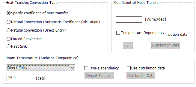
Sets the heat transfer between boundary and outer environment.

The heat flux due to the heat transfer is calculated by the surface temperature θ, room (ambient) temperature θroom, and the related coefficients.

Heat Transfer: Convection Type

Setting Item	Notes
Specify Coefficient of Heat Transfer	Sets the value (h) directly. The heat flux from boundary to environment is h(θ-θroom) By selecting [Use distribution data], the coefficient of heat transfer is set with the user-defined distribution. Click the [Distribution Data] button to open the dialog box. See [How to Set Distributed Boundary Condition and Body Attribute] for the detail. Select [Temperature Dependency] in order to set the coefficient of heat transfer with temperature dependency in the the [Temperature-Coefficient of Heat Transfer] table , if clicked, open the [Edit Nonlinear Table] dialog box to edit the data. In the case of forced convection, select [Forced Convection] and enter the air flow speed and the characteristic length. If you want to manually set the coefficient of heat transfer of forced convection, see [Coefficient of Heat Transfer of Forced Convection].
Natural convection (automatic calculation)	Calculates the heat transfer to the environment by natural convection. The heat flux from boundary to environment is calculated as below. con(θ-θroom)^(5/4) where con is automatically calculated by con = 2.51 x C x (1/L)^(1/4) C and L are given by Table 1, which are "Vertically placed board", "Horizontally placed board with the hot face up" and "Horizontally placed board with the hot face down" To use this boundary condition, the model must be oriented so that the negative Z direction points to the ground. Please note that the direction is critical for the natural convection.
Natural convection (Direct Entry)	Calculates the heat transfer caused by natural convection. The coefficient con is not calculated automatically. The heat flux from the boundary to the environment is calculated with the specified coefficient con as below. con(θ-θroom)^(5/4)
Forced convection	Calculates the heat transfer to environment by forced convection. Given the air flow speed (V) and the characteristic length (L) , the coefficient of heat transfer (h) is calculated by: h = 3.86 x (V/L)^(1/2) See "Coefficient of forced convection" for more information. The heat flux from boundary to environment is calculated as below. h(θ-θroom) See [Simple Fluid-Thermal Analysis] or [Fluid-Thermal Analysis] for the coefficient of heat transfer of forced convection.
Heat sink	Directly specifies a thermal resistance value R in the dissipation to the ambient. Thermal resistance value is an indicator of the dissipation capability of heat sink. It is expressed as follows where h is a coefficient of heat transfer and S is an area. R = 1 / (h * S) R is converted by this equation to h. Select [Temperature Dependency] in order to set the thermal resistance, R, with temperature dependency in the the [Temperature-Thermal Resistance] table. , if clicked, open the [Edit Nonlinear Table] dialog box to edit the data.

Room (ambient) temperature

Specifying Method

Notes

Use ambient temperature of the analysis condition

Uses the ambient temperature set on the [Thermal analysis tab].

Direct Entry

Specifies the room (ambient) temperature.

For transient analysis, the change of ambient temperature over time can be set by selecting Time Dependency.

By clicking Weight Function, the [Time-Weight] table will show up.

By selecting Use distribution data, the room (ambient) temperature is set with the user-defined distribution.

Click the Distribution Data button to open the dialog box.
See [How to Set Distributed Boundary Condition and Body Attribute] for the detail.

Thermal Resistance

The thermal resistance can be set on a face (or on an edge in 2D) where two bodies meet.

The thermal resistance will be distributed evenly on all the specified faces.

There are three types to define the thermal resistance.

All Thermal Resistance: R [deg/W]

Thermal Resistance per Area: Rs[m2 deg/W]

Thermal Conductivity and Thickness: λ[W/m/deg] and d[m]

The relationship of these types are expressed as follows where S[m2] is the area of boundary condition face.

R [deg/W] = Rs / S = d / (λS)

When executing electric-thermal analysis (Coulomb/Watt) or thermal-stress analysis (Watt/Galileo),

the boundaries are conditioned as follows:

Bond is default when coupled with stress analysis

unless "Separate in stress analysis" is selected.

Conductive is default when coupled with electric analysis

unless "Insulate in electric analysis" is selected.

Select [Temperature Dependency] in order to set the coefficient of heat transfer with temperature dependency either in the [Temperature-Thermal Resistance] table for [All Thermal Resistance]/[Thermal Resistance per Area]

or in the [Temperature-Thermal Conductivity] table for [Thermal Conductivity and Thickness].

, if clicked, open the [Edit Nonlinear Table] dialog box to edit the data.

Bond	The faces are bonded.
Separate	The faces are off contact completely. They don't interact each other. One might penetrate the other depending on the loading direction.
Conductive	The faces are bonded and the current flows across the faces.
Insulated	No current flows across the faces.

Thermal resistance cannot be specified when coupled with electromagnetic analysis (Hertz) or magnetic analysis (Gauss).

Measuring Terminal

Table of temperature can be output. It will not affect the analysis results of temperature distribution.

The maximum, minimum and average temperatures of the specified area are output for the boundary temperature in the output table.

It can be added as a terminal in the equivalent circuit for [heat flow rate] or [thermal resistance] in the output table.

It can be added as a selection candidate of the boundary for [Junction-thermal resistance between boundaries]

See the technical note [Result Table in the Thermal Analysis] for the details of the output items.

Measuring terminal boundary condition is treated as follows in the thermal analysis.

	Without Outer Boundary Conditions Setup	With Outer Boundary Conditions Setup
Outer Face of Model	Adiabatic	Boundary condition set in the [Outer Boundary Conditions]
Inner Face of Model	Not applicable	Not applicable

No Setting (Adiabatic)

Sets the adiabatic wall.

It is required to be set on the outer wall of the model.

If it is set on the internal wall, it will not function as adiabatic.

If you want to set adiabatic face inside the model, select "Discontinuous" on [Symmetry/Continuity] tab.

Usually, there is no heat transfer but if [Ambient (speed prioritized)] or [Surface-to-surface (accuracy prioritized)] is selected for the radiation setting, the heat transfer due to the radiation will be generated.

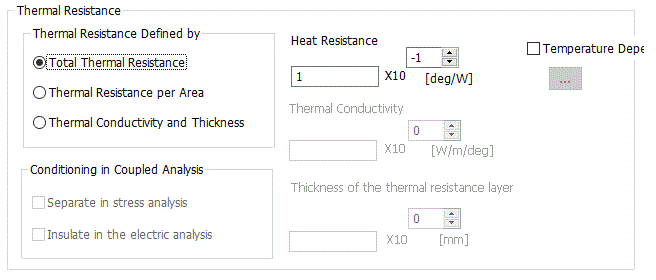
Radiation Setting

The emissivity can be set at [Radiation Setting] for analysis condition.

Radiation Type	Notes
None	Does not take the radiation from the surface into account.
Ambient (speed prioritized)	Takes into account the radiation from the surface to the environment outside the model. The radiation to other surface is not taken into account. The radiation energy transmits through other objects. It is assumed that the model is entirely surrounded by the ambient face with no obstacle in between. (View factor = 1). Given the emissivity (ε), The heat flux from the surface to the environment is calculated as below. 5.68 * 10^-8 * ε * (θ^4-θroom^4) where θ is surface temperature of the boundary and θroom is room (ambient) temperature. For the emissivity, the default value of the [Thermal Analysis tab] or the value of the [Thermal Surface tab] of body attribute with boundary condition is used. To use other temperature, select Individual Setting, click and set up at [Indivaidual Radiation Setting]. Typically, the ambient temperature set on the [Thermal Analysis tab] is used for the ambient radiation temperature. To use other temperature, select Individual Setting, click and set up at [Indivaidual Radiation Setting]. Note: If the view factor is not 1 due to the obstacles, concave radiation surface, or closed space, use [surface-to-surface].
Surface-to-surface (accuracy prioritized)	Takes into account the radiation between the surfaces that are set with this setting. The radiation from the surface to the environment outside the model is also taken into account. Select this option to calculate the radiation between the distant objects or in the closed domain. It takes longer time than the [ambient] because this calculation requires radiation surface check, calculation of view factor, and calculation of heat transfer across the surfaces. See [Radiation: Equations and Setting Method] for the details. For the emissivity, the default value of the [Thermal Analysis tab] or the value of the [Thermal Surface tab] of body attribute with boundary condition is used. To use other temperature, select Individual Setting, click and set up at [Indivaidual Radiation Setting]. Typically, the ambient temperature set on the [Thermal Analysis tab] is used for the ambient radiation temperature. To use other temperature, select Individual Setting, click and set up at [Indivaidual Radiation Setting].
Follow the outer boundary condition	Applies the same radiation setting of the outer boundary condition.

Other Options

Options

Notes

Uniform Temperature

Sets the uniform temperature on the boundary.

The faces having the same boundary condition name are to have the same temperature even if they are physically separated.

Uniform temperature represents the situation where the faces are in contact with the material having infinite high thermal conductivity.

You may apply Uniform temperature on the boundary where metals having quite high thermal conductivities exist.

See Example 12: Uniform Temperature Boundary Condition of thermal analysis.