


|
Home / How to Set Body Attribute, Material Property and Boundary Condition / Boundary Condition Tabs / Mechanical Tab
Mechanical Tab
Boundary conditions relating to mechanicals are set on this tab.
It is in the [Edit Boundary Condition] dialog box. See [How to Set Boundary Condition].
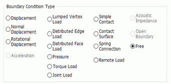
The links in the boundary condition type below lead to their setting details.
|
Boundary Condition Type |
Notes |
||||||||||||||||||||||
|
Specifies the displacement constraint. Select the directions to constrain the displacement and enter the values. If 0 is entered in a direction, there will be no displacement in that direction. For the forced displacement, enter the displacement value.
If [Constrain the freedom of shells] is selected on the analysis condition, the rotation can be constrained too.
Select [Use distribution data] to define the distribution.
|
|||||||||||||||||||||||
|
Sets the displacement normal to the set face. It sets the normal displacement without constraining the displacement in the inward direction of the face.
To fix a displacement, enter 0. For the forced displacement, enter the displacement value.
|
|||||||||||||||||||||||
|
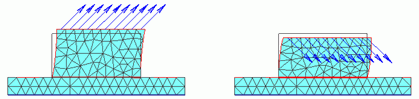
Specifies the rotation angle around the specified axis. The axis is defined by Coordinates on Axis and Vector of Axis. For the positive angle, the rotational direction is clockwise with reference to the axial vector. It is counter-clockwise for the negative angle.
Displacement in the rotation axis direction and radius direction are not constrained. Like torque load, the load is observed only in the rotational direction. The trace may not become arc as the displacement in the radius direction is not constrained.
If [Rotate at constant radius] is selected, If [Constrain displacement in axis direction] is selected,
|
|||||||||||||||||||||||
|
Sets the acceleration vector on the set face.
If [Constrain the normal displacement] is selected,
|
|||||||||||||||||||||||
|
Applies the lumped load on a vertex If [Constrain the freedom of shells] is selected in the [Analysis Condition Setting] dialog box, rotational force or moment can be applied.
|
|||||||||||||||||||||||
|
Sets the distributed edge load by the load per unit length [N/m] in any direction. Alternatively you may select "Set the total load" and enter the total load [N] instead of the load per unit length. The total load will be distributed evenly to all the edges selected for the boundary.
|
|||||||||||||||||||||||
|
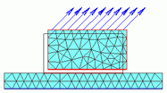
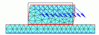
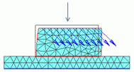
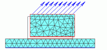
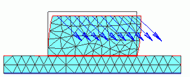
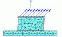
Sets the distributed face load by the load per unit area [N/m2] in any direction. Alternatively you may select [Set the total load] and enter the total load [N] instead of the load per unit length. The total load will be distributed evenly to all the faces selected for the boundary. The list below indicates the possible topologies and how the total load is distributed when selected.
If [Set the total load] is deselected, you can define the distribution by selecting [Use distribution data]. If [Constrain the freedom of shells] is selected in the [Analysis Condition Setting] dialog box, rotational force or moment can be applied.
|
|||||||||||||||||||||||
|
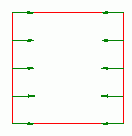
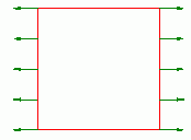
Sets the pressure on the face (or edge in 2D). The normal and inward direction onto the face (edge) is defined positive as shown below.
Alternatively you may select [Set the total load] and enter the total load [N] instead of the load per unit length. The load will be distributed evenly to all the faces selected for the boundary. If [Set the total load] is deselected, you can define the distribution by selecting [Use distribution data]. See "Options for Mechanical Boundary Condition" below
|
|||||||||||||||||||||||
|
Specifies the torque load around the specified axis. If the torque is positive, its direction is clockwise with reference to the axial vector. If the torque is negative, the direction is counter-clockwise. The axis is defined by Coordinates on Axis and Vector of Axis. The torque can be applied on vertex, edge or face. The same-name torque can be applied on multiple number of vertices, edges or faces. In that case, the average distance from the rotation axis is calculated, and the load [N] is the torque [Nm] divided by the average distance. The same-name torque can be used for the same type of topologies.
|
|||||||||||||||||||||||
|
Joint Load |
Sets the attractive load or the repulsive load to the joint load boundary pair. The joint load boundary conditions are paired on the [Boundary Pair] of [Analysis] to set the joint load value. See [Joint Load Boundary] for the [Constrain except axial direction] option, which simulates the actual constraint imposed by a bolt.
|
||||||||||||||||||||||
|
Analyzes the behaviors of two bodies meeting on a face (or on an edge in 2D).
There are 6 types of contacts. In the simple contact, slip, off contact, and automatic judgment (1.coefficient of friction: zero, no peeling, 2.with friction, 3.with peeling) are selectable. Bond requires no setting. It is equivalent to the state with no boundary condition (no constraint).
Specify the right one for your analysis.
|
|||||||||||||||||||||||
|
Specifies the faces subject to the contact analysis as contact surface. It will be either the contactor surface or the contactee surface.
If one is designated as contactor, the other should be contactee. Their boundary conditions need to be paired on the the Boundary Pair dialog. When the friction is taken into account, set the coefficient of friction during the pairing.
|
|||||||||||||||||||||||
|
Spring Connection |
Generates the spring force according to the relative deflection of the spring connection boundary pair. The spring connection boundary conditions are paired on the [Boundary Pair] dialog box of [Analysis] to set the spring constant type and the values of the components.
|
||||||||||||||||||||||
|
Remote Load |
Takes into account the distributed load and the torque load between the remote point and the boundary. Its results are equivalent to those of the distributed load and torque load combined. Contributes to simplifying the analysis model. Requires the setting of the coordinates of the remote point and the setting of the load.
|
||||||||||||||||||||||
|
Acoustic Impedance |
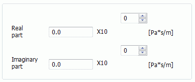
Takes into account the influence of the surrounding medium such as air and water. Refer to Terminology in Acoustic and Piezoelectric Analysis. Requires to be set so that the results of analysis and experiment match. Alternatively, a method in Example 23: Air Damping of Cantilever can be used as well. Available in the piezoelectric solver, but ignored in the static analysis. Not allowed to use unless the piezoelectric-transient analysis or the transient analysis using resonant mode is selected. Used to analyze the resonant mode if the piezoelectric-transient analysis or the transient analysis using resonant mode is selected. Not available in the stress analysis.. |
||||||||||||||||||||||
|
Open Boundary |
Available for the piezoelectric analysis. See Open Boundary Tab. Also see Example 16 of Piezoelectric Analysis and a technical note [PML]. Not available in the stress analysis.. |
||||||||||||||||||||||
|
Free |
Mechanically no constraint at all. |
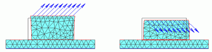
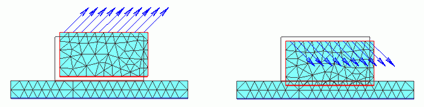
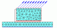
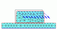
Options for Mechanical Boundary Condition
|
Setting Items |
Notes |
|
Time Dependency |
Selectable in the stress analysis if
the transient analysis or the static analysis is selected for [Analysis type], and [Multi step/Multi-step thermal load analysis] is selected on the Step/Thermal Load tab.
Select Time Dependency and click Weight Function. [Time-Weight] table
Transient analysis is available in an optional package.
|
|
Set ON/OFF |
Selectable in the stress analysis if
[Analysis type] is static analysis, and [Multi step/Multi-step thermal load analysis] is selected on the Step/Thermal Load tab.
It can be set if the boundary condition type is displacement, normal displacement, rotational displacement,
It can set or remove boundary condition at the specific step in the multi-step analysis/multi-step thermal load analysis. Select Set ON/OFF, and click ON/OFF List. You can confirm time, step, Initial temperature and reached temperature. Also, you can confirm the weight function which is created by the setting at ON/OFF setting.
If the boundary condition type is displacement, normal displacement, or rotational displacement,
If the boundary condition types are lumped vertex load, distributed edge load, distributed face load, pressure, or torque load,
It can be used together with the setting of time dependency (weight function). |
|
Uniform Displacement |
Sets the boundary to have the uniform displacement. It can be set in UX, UY and UZ directions individually. The faces having the same boundary condition are to have the same displacement even if they are physically separated.
If "Constrain the freedom of shells" is selected on the analysis condition,
This is applicable, for example, for the boundary where a very hard material is pressed.
|
|
Rigid Face |
Select the rigid face boundary condition. If selected, it allows all the selected faces to belong to the same rigid body, resulting in zero relative displacement. The rigid body attribute serves in a similar way. For the details, please refer to the Analysis Domain tab.
|
|
Use Distribution Data |
Selectable for Displacement, Distributed face load (total load deselected), and Pressure.
In the case of Displacement
Use distribution data
In the case of Distributed face load
Use distribution data
In the case of Pressure
Use distribution data
Click the Distribution Data button to open the dialog box. |