Home / How to Set Analysis Condition / List of Analysis Condition Tabs / Transient Analysis Tab

Transient Analysis Tab

Analysis conditions for the transient analysis are set on this tab.

It is in the [Analysis Condition Setting] dialog box. See also [How to Set Analysis Condition].

Setting Item

Notes

Timestep

Manual

Higher Accuracy

The number of calculation steps, the output interval, and the timestep are specified in multiple rows.

The calculation time equals to number of calculation steps multiplied by timestep [s].

Number of Calculation steps	Timestep
20	0.05
40	0.025

The total calculation time is as follows:

20x0.05 + 40x0.025 = 2.00[s]

If [Specify the output interval] is selected, an output interval can be specified for each row.

It can limit the output result and downsize the result file.

Number of Calculation steps	Output interval	Timestep
20	1	0.05
40	2	0.025

If all the output intervals are set to 1, the number of results will be 20 + 40 = 60. As the output intervals above are set to 1 and 2, the number of results will be 20 + 20 = 40.

* Too large timesteps might degrade the accuracy.

In such a case, retry with smaller timestep.

* To add rows, click a cell in the last row or press the return key on a row before the last.

[Manual] for the timestep can not be applicable for the analysis conditions below.
Electromagnetic-Transient Analysis
Constant Rotation Speed for Rotating Machinery in Magnetic-Transient Analysis
Translational Machinery in Magnetic-Transient Analysis

If [Higher Accuracy] is selected, calculation with the timestep divided into smaller elements can increase its accuracy.

This is available for the stress and fluid analyses.

In [Detailed Automatic Timestep Setting] with [If non-convergence, set a finer timestep] selected, if a calculation does not converge, set the timestep finer and redo the calculation.

If [Adjust referring to Courant number] is selected in [Detailed Automatic Timestep Setting], the timestep is calculated such that the flow travel distance per time meets the requirement associated with the specified Courant number.

[Maximum Number of Divisions per Step] must be selected.

Calculation is aborted when the maximum number of divisions is exceeded.

For the detail of [If non-convergence, set a finer timestep], refer to the corresponding help menu of the [High-Level Setting Tab].

Automatic

For the details, please refer to the Transient Analysis Tab (Automatic).

[Number of Calculation Steps] to be an integer equal to or greater than 1.

[Output interval] to be an integer equal to or greater than 1.

[Timestep] to be a real number greater than 0.

Click the Table button. The Time Table window will appear.

You can see the weight function set on Mechanical tab, Thermal tab or Electric tab of boundary condition, or Heat Quantity tab of body attribute.
See [Weight Function Setting].

Steady-state mode in the magnetic transient analysis.
If [Steady-state analysis] is selected, the transient analysis is executed with a step of 1.
Steady-state current is only allowed as an input current. The analysis type is practically a steady-state analysis.

Restart

Select Continue from the last session to restart the calculation from the last calculated step.

Not available for the magnetic and acoustic analyses, and the transient analysis using resonant mode in the piezoelectric analysis.

Initial Temperature

Sets the initial temperature of the whole model in the thermal transient analysis. The temperature of the model changes with time.

If Use distribution data is opted,
the initial temperature will be distributed over the model.

Click the Distribution Data button to open the dialog box.
See [How to Set Distributed Boundary Condition and Body Attribute] for the detail.

Initial Velocity

Available for the stress-transient analysis.

The initial velocity can be set on each body attribute individually too.

If "Use distribution data" is selected,
the initial velocity will be distributed over the model.

Click the Distribution Data button to open the dialog box.
See [How to Set Distributed Boundary Condition and Body Attribute] for the detail.

(Note) The stress transient analysis is available in an optional package.

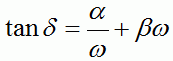
Coefficients of Rayleigh Damping

Available for the stress-transient analysis.

They can be set on each body attribute individually too.

If Rayleigh damping is considered to be the damping effect on the frequency component of vibration,
Mechanical loss tangent (tanδ) is expressed with angular frequency ω as follows. (Refer to [Mechanical Damping] for derivation of equations.)

Click Frequency-Mechanical loss tangent Graph to see the frequency response of mechanical loss tangent,

where α is damping of low frequency vibration and β is damping of high frequency vibration.

By setting β, you can remove noise of high-frequency vibration.

The detail of the coefficient of Rayleigh damping is explained at [Stress Transient Analysis] and [Mechanical Damping] in the Technical Notes.

(Note) The stress-transient analysis is available in an optional package.

Solution Method

Time-directional solution method is selected for the acoustic analysis.

Explicit method and implicit method are available. The explicit method is an accuracy-oriented solution, and the implicit method is a speed-oriented solution.

High-speed mode is selectable in the explicit method. In the high-speed mode, the domain where the field does not propagate is automatically removed from the analysis domain to allow the higher calculation speed.

The threshold value to judge the propagation of the field can be set by the tolerance.

The threshold value is the largest flux (acoustic intensity) with tolerance.