
CAE Software【Femtet】Murata Software Co., Ltd.
Example8 Heat Radiation by Forced Convection(Transient Analysis)
General
-
The model is the same as Exercise 7: A heat source is placed on a substrate, and there is a forced air flow for cooling in parallel to the substrate. The heat radiation is analyzed under the transient condition.
-
The heat transfer coefficient is acquired manually.
To acquire it automatically, see “Ex.1 of Simple Fluid-Thermal Analysis”.
-
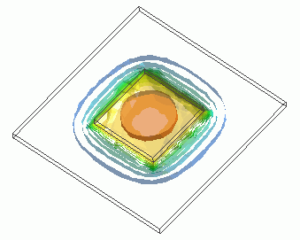
The temperature distribution and the heat flux vectors are solved.
-
Unless specified in the list below, the default conditions will be applied.
Analysis Space
|
Item |
Settings |
|
Analysis Space |
3D |
|
Model unit |
mm |
Analysis Conditions
|
Item |
Settings |
|
Solver |
Thermal Analysis [Watt] |
|
Analysis Type |
Transient analysis |
|
Options |
N/A |
The transient analysis is set up as follows. The total number of steps is 20. The time step is 30 second.
Therefore, the temperature distributions for 600 seconds are solved.
|
Tabs |
Setting Item |
Settings |
||||||||
|
Transient analysis |
Table |
|
||||||||
|
Initial Temperature |
25[deg] |
Model
The same as Exercise 7. The material properties and the boundary conditions are the same as well.
The substrate (VOL1) and the heat source (VOL2) are created as solid body box, and the heat amount is defined in the body attribute of VOL2.
The heat transfer coefficients for the top and bottom faces of the substrate and the top face of the heat source are calculated basede on the simplified equation.
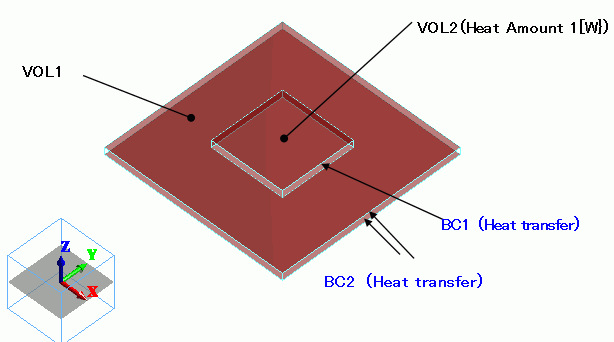
Body Attributes and Materials
|
Body Number/Type |
Body Attribute Name |
Material Name |
|
0/Solid |
VOL1 |
006_Glass_epoxy * |
|
1/Solid |
VOL2 |
001_Alumina * |
* Available from the Material DB
The heat source of VOL2 is set up as follows.
|
Body Attribute Name |
Tab |
Settings |
|
VOL2 |
Heat Source |
1[W] |
Boundary Conditions
The heat transfer coefficients for the forced convection are calculated as follows. For the details, please refer to the Heat Transfer Coefficient for Forced Convection
To acquire it automatically, see “Ex.1 of Simple Fluid-Thermal Analysis”.
h = 3.86 x (V/L)0.5xC [W/m2/deg]
where
Air flow V=1[m/s]
On the top and bottom faces of VOL1: Characteristic length L=0.05, C=1 -> h=17.26
Top face of the heat source (VOL2): Characteristic length L=0.02, L’=0.015, C=1 * -> h=27.3
*
The thickness (d) of the speed boundary layer at the edges of the heat source is calculated as follows
d=0.0182x(L’/V)0.5= 2.3[mm]
This is close enough to the thickness of heat source, so we set C=1.
|
Boundary Condition Name/Topology |
Tab |
Boundary Condition Type |
Settings |
|
BC1/Face |
Thermal |
Heat Transfer/Ambient Radiation |
Heat transfer coefficient: 17.26 [W/m2/deg] Ambient temperature: 25[deg] |
|
BC2/Face |
Thermal |
Heat Transfer/Ambient Radiation |
Heat transfer coefficient: 27.3 [W/m2/deg] Ambient temperature: 25[deg] |
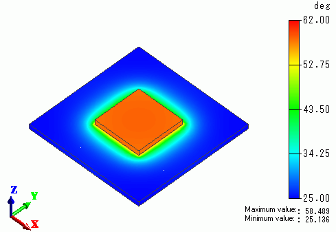
Results
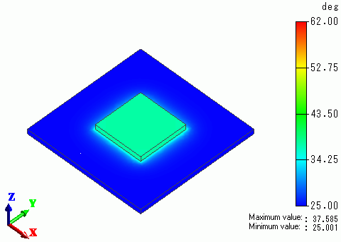
The temperature distributions at each time are shown below.
At Minimum/Maximum Value on the Contour tab of [Graphics Setup], deselect “Automatic” and set 25 => 62.
In 60 seconds
In 180 seconds
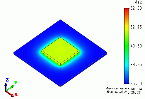
In 360 seconds
The temperature vs. time is plotted for the center of the heat source.
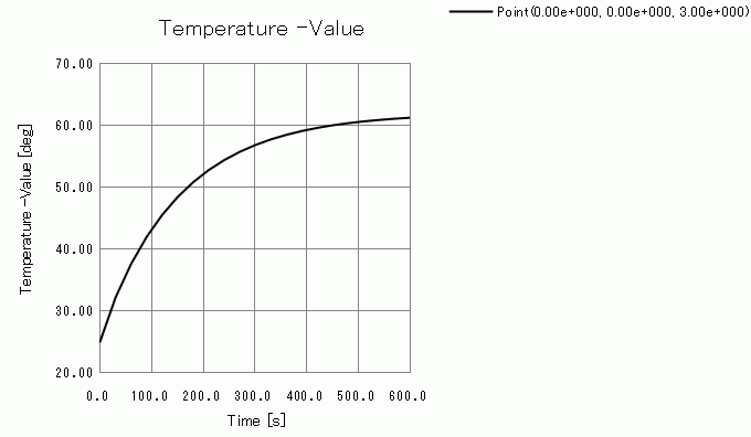
It is getting stabilized in 600 seconds.