Example20 Further Analysis with Saved Temperature Data (Transient Analysis)

General

Further analysis is performed for Exercise 4 Heating due to the Iron Loss (Temperature-Dependent Materials) of Magnetic Field – Thermal Coupled Analysis with the result data used as the initial temperature.
At the end of Exercise 4, save the results data in a csv file by “Output Node Results by CSV” on Exercise 4. See [ Right-Click Menu for Results Window]. The saved csv file is imported for this exercise.
See [How to Set Distributed Boundary Condition and Body Attribute] for more information.
The temperature distribution and the heat flux vectors are solved.
Unless specified in the list below, the default conditions will be applied.

Analysis Space

Item	Setting
Analysis Space	3D
Model unit	mm

Analysis Conditions

Item	Settings
Solver	Thermal Analysis [Watt]
Analysis Type	Transient analysis
Options	None

The Transient Analysis tab is set up as follows. The total number of steps is 20. The time step is 30 second.
Therefore, the temperature distributions for 10 minutes are solved. The initial temperature is the result of Exercise 4 of magnetic field – thermal coupled analysis.

Tabs

Setting Item

Settings

Transient analysis

Table

Number	Calculation steps	Output steps	Time step [s]
1	20	1	30

Initial Temperature

Select “Use distribution data”.

Distribution Dimension: 3D

[Coordinates-Temperature] Table

Temperature Distribution Data

* The csv file saved in advance is used:
Right click on results window
> select “Output Node Results by CSV”
Note that only numerical data are extracted.

Model

Basically the same as Exercise 4: Heating due to the Iron Loss (Temperature-Dependent Materials),

except that “Air” is removed as it is not needed.

Body Attributes and Materials

Body Number/Type	Body Attribute Name	Material Name	Mesh Size
5/Solid	Coil2	008_Cu *	1
7/Solid	Coil1	008_Cu *	1
6/Solid	Core	Core	2

* Available from the Material DB

The material properties of the core are set up as follows.

Material Name	Tab	Settings
Core	Thermal Conductivity	Thermal Conductivity: 10[W/m/deg]
	Density	Density: 7000[kg/m3]
	Specific Heat	Specific heat: 800[J/Kg/deg]

Boundary conditions

Select “Natural convection (automatic calculation)” on the outer boundary condition.

Boundary Condition Name/Topology

Tab

Boundary Condition Type

Settings

Outer Boundary Condition *

Heat

Heat Transfer/Ambient Radiation

Natural convection (automatic calculation)

Room temperature: 25[deg]

To set Outer Boundary Condition, go to the [Model] tab

and click [Outer Boundary Condition] .

* The correction coefficient for the natural convection is calculated automatically. See [Heat Transfer/Ambient Radiation] for more information.

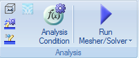
How to view the distribution

Click “Run Mesher” on the pull-down menu of [Run Mesher/Solver] and see the meshing result.

Select “Distributed initial temperature” at [Field] to view the entered distribution.

You may click “Run Mesher/Solver” instead. In that case, select “Mesh Information” at [Mode] and then select “Distributed initial temperature” at [Field].

Results

The temperature distributions in 30s, 300s and 600s are shown below.
The scale of color scale is fixed to 20[deg] – 90[deg].

The temperature of Core goes down over time.

Temperature distribution in 30s

Temperature distribution in 300s

Temperature distribution in 600s

See other Thermal Analysis examples.