The calculation results are available in various format.
Let's see the field vectors, and some graphs and charts.
-
Check the calculated values.
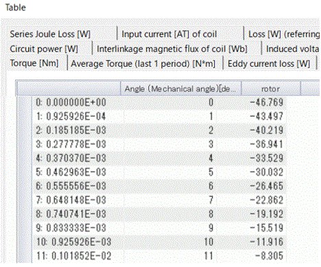
The results such as torque and interlinkage magnetic flux of coil are summarized on tables.
-
In the 2D analysis, interlinkage magnetic flux of coil and various current values are positive in -Y direction.
-
Table can be seen by clicking 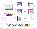 [Table] [Table]  on the [Results] tab. on the [Results] tab.
The values in the table can be copied and pasted, or exported in CSV.
|
|
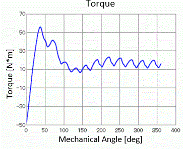
- Show a graph of torque.
Select [Torque] tab in the table and click  . .
|
|
|
-
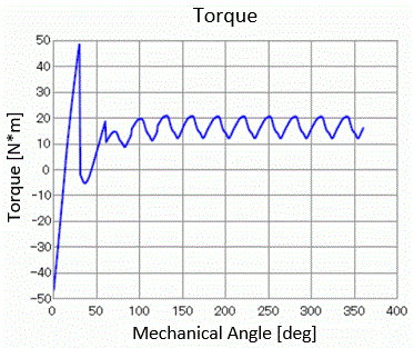
In this tutorial, the calculation is performed up to 360 steps (mechanical angle: 360[deg) but the torque is not in the steady state.
In order to obtain the actual torque of motor, it is needed to increase the number of steps till the torque reaches the steady state.
As the input is by voltage, the coil current is in the transient state in the initial stages. It will be some time before it reaches the steady state.
In the case of input by current, the coil current is in the steady state from the beginning.
-
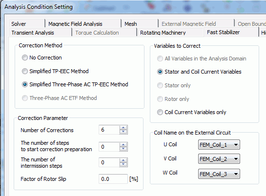
Fast stabilizer realizes the steady state with small number of steps in some cases.
The diagram on the right shows the settings and results in this tutorial.
Torque reaches the steady state at about 150 [deg].
Refer to the [Fast Stabilizer Tab] for more information.
|
|
-
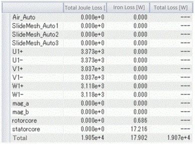
View Joule loss of the coil and iron loss of the core.
Select [Loss [W] (referring to value over 1 period from the final step)] tab.
|
|
-
Close table.
|
|
-
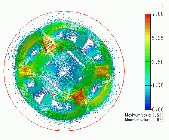
Let's see the vectors of magnetic flux density.
On the [Results] tab, go to

initial setting of the field  is [Magnetic flux density]. is [Magnetic flux density].
Click [Element Vector] . .
The vector diagram of magnetic flux density will show up.
-
Although the model is a half symmetric, the results are shown for the full model. It is switchable by  . .
-
The setting for the results display can be registered for later reference.
The setting can be easily applied to other results.
See [Registering Results Display Setting].
|
The Vectors of Magnetic Flux Density |
|
-
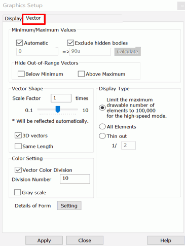
To modify the shape of vectors,
on the [Results] tab, go to
and click [Graphics Setup]  . .
In the [Graphics Setup] dialog box,
select the [Vector] tab,
and modify the magnitude and the shape of vectors.
The Vector tab is explained here
|
|
-
Next, we will show the contour diagram of magnetic field at the 80th step.
On the [Results] tab, go to
and set mode  [80:0.740741E-02], and field [Magnetic field [A/m]]. [80:0.740741E-02], and field [Magnetic field [A/m]].
Then click [Gradation contour diagram] . .
The contour diagram of magnetic field will be shown.
|
|
- If you click [Displacement Outline]
 , a graph will show up which reflects the rotor's rotation. , a graph will show up which reflects the rotor's rotation.
|
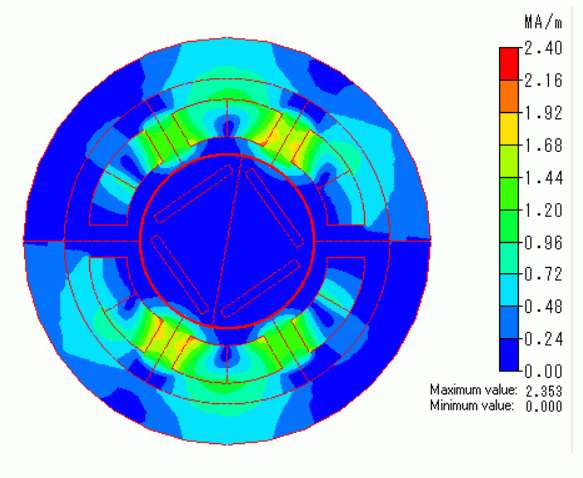
Contour diagram of the magnetic field |
|
|
|
-
Various results can be shown by [Show Results] on the [Results] tab.
- See value at the specific coordinates: Click [Results at Specified Coordinates]
 . .
- Create graph: Click [Display Graph]
 . .
- Display in animation: Click [Create Animation]
 . .
|
|


 Prev Next